Synchronization and Detection in MIMO Systems
Introduction
The first approach to carrying out space-time processing of data sampled at an array of sensors dates back to the second world-war (the Bartlett beamformer), and was an application of Fourier-based spectral analysis to spatio-temporally sampled data. Space-time processing emerged as a field of interest, because, at the time, source localization was an imminent problem to radar and sonar applications.
Nowadays, the ever growing demand for mobile communications is constantly increasing the need for better coverage, improved capacity and higher quality service. Space-time processing promises to improve mobile radio performance significantly. The principles of space-time processing can be used to develop 'smart' antennas that use adaptive arrays of antenna sensors. Therefore, the 'smart' antenna concept has become very interesting to the mobile communications industry.
This tutorial gives an overview of the basic principles and the current state of research in 'smart' antennas. Note, that throughout the report narrowband communication systems are assumed. Wideband communication systems like CDMA are not discussed here!
The document is organized in the following manner. Section 1 is a brief introduction to the subject of 'smart' antennas. Firstly, the basic principle behind 'smart' antennas is explained using a simple, but insightful example. Afterwards, the advantages of using 'smart' antennas in wireless communication systems are discussed. Some mathematical preliminaries concerning the treatment of narrowband signals are introduced in Subsection 1.3. The presentation of a fading channel model appropriate for 'smart' antenna systems follows in Section 2. Section 3 presents signal processing algorithms that are used in the Uplink (mobile to base station) of a wireless communication system. Similarly, Section 4 presents algorithms that are used in the Downlink (base station to mobile radio).
1.1 Basic principle
The diagram of Figure 1 shows the principal system elements of a 'smart' antenna system. The 'smart' antenna consists of the sensor array, the patternforming network and the adaptive processor:
Sensor Array
The sensor array consists of N sensors designed to receive (and transmit) signals. The physical arrangement of the array (linear, circular, etc.) is arbitrary, but places fundamental limitations on the capability of the 'smart' antenna
Patternforming Network
The output of each of the N sensor elements is fed into the patternforming network, where the outputs are processed by linear time-variant (LTV) filters. These filters determine the directional pattern1 of the 'smart' antenna. The outputs of the LTV filters are then summed to form the overall output y(t). The complex weights of the LTV filters are determined by the adaptive processor
Adaptive processor
The adaptive processor determines the complex weights of the patternforming network. The signals and known system properties used to compute the weights include the following items, details of which are discussed in Sections 3 and 4 about Uplink and Downlink Processing:
- The signals received by the sensor array, i.e. xk(t) for k = 1 ¼N
- The output of the 'smart' antenna, i.e. y(t)
- The spatial structure of the sensor array
- The temporal structure of the received signal
- Feedback signals from the mobiles
- Network topology
The working principle of a 'smart' antenna is now explained using a simple example. In the example, the sensor array is assumed to be a uniform linear array (ULA) consisting of 2 identical omnidirectional sensors as shown in Figure 2.
Example
Assuming that a signal s(t) is generated by a mobile radio located in the
far-field of the 'smart' antenna, the electromagnetic wave
arriving at the sensor array is approximately plane (see Figure
2). If the direction
q is different from zero, then sensor 2 experiences a time delay with
respect to element 1 of
where d is the sensor spacing and v is the velocity of the plane
wave. If s(t) is a narrowband signal with carrier frequency f
0,
then the time delay t corresponds to a phase shift of
where l
0 is the wavelength corresponding to the carrier
frequency, i.e.
Now assume that a second interfering signal n(t) with the same
carrier frequency impinges on the array. The directions of s(t) and
n(t) are 0 radians and [(p)/6] degrees, respectively. The
task of the 'smart' antenna is to null out the interfering signal such
that the output becomes s(t).
In this example, the
patternforming network is reduced to two
complex weights, w
1 = w
1,1 + jw
1,2 and w
2 = w
2,1 +jw
2,2. Then the 'smart' antenna output due to s(t) is
|
s(t){[w1,1 + w2,1] + j[w2,1 + w2,2]} |
| (4) |
For a sensor spacing d = l
0/2, the interfering signal
n(t) exhibits a phase lag of p/2 at sensor 2 with respect to
sensor 1. Hence the output of the 'smart' antenna due to n(t) can be
written as
|
n(t)exp(jp/4)[w1,1 + jw1,2] +n(t)exp(-jp/4)[w2,1 + jw2,2] |
| (5) |
So for the array output to be equal to s(t), it is necessary that
|
|
|
| |
|
| |
w1,1 - w1,2 + w2,1 + w2,2 |
|
|
| |
w1,1 + w1,2 - w2,1 + w2,2 |
|
|
| (6) |
|
Solving equation (
6) yields:
|
w1,1 = |
1
2
|
, w1,2 = |
1
2
|
, w2,1 = |
1
2
|
, w2,2 = - |
1
2
|
|
| (7) |
The normalized
directional pattern in decibels for an N-element ULA
with single complex co-efficient LTV filters is given by
|
G(q) = 10log10 | ì
ï
í
ï
î |
ê
ê
ê
ê
ê
|
N-1
å
k=0
|
wkexp([(j2pkdsin(q))/(λ0)]) |
wHw
|
ê
ê
ê
ê
ê
|
2
|
ü
ï
ý
ï
þ
|
|
| (8) |
Figure
3 shows the normalized
directional pattern of
the two-sensor
'smart' antenna without any weighting in the
patternforming network.
Figure
4 shows how the
directional pattern
changes, when the weights of equation (
7) are used instead.
It is seen that now
a null is placed exactly at an azimuth of [(p)/6] radians, the
direction of the interferer. Additionally, there is no signal
attenuation at 0 radians, the direction of the desired signal. Therefore
it can be said, that the 'smart' antenna is capable of separating the
desired signal s(t) and the interfering signal n(t).
|
|
Figure 3: Normalized directional pattern of the non-weighted sensor array
|
|
|
Figure 4: Normalized directional pattern of the weighted sensor array
|
1.2 Performance improvements
| |
Figure
Figure 5: Channel Re-use via Angular Separation
|
| |
| |
Figure
Figure 6: Channel Re-use via Spatial Separation
|
| |
A space-time processor ('smart'antenna') is capable of forming
transmit/receive beams towards the mobile of interest. At the same
time it is possible to place spatial nulls in the direction of
unwanted interferences. This capability can be used to improve the
performance of a mobile communication system:
- Increased antenna gain
- The 'smart' antenna forms transmit
and receive beams as shown in Figure 5. Therefore, the 'smart'
antenna has a higher gain than a conventional omni-directional
antenna. The higher gain can be used to either increase the effective
coverage, or to increase the receiver sensitivity, which in turn can
be exploited to reduce transmit power and electromagnetic radiation in
the network.
- Decreased inter-symbol-interference (ISI)
- Multipath
propagation in mobile radio environments leads to ISI.
Using transmit and receive beams that are directed towards the mobile
of interest reduces the amount of multipaths and ISI.
- Decreased co-channel-interference (CCI)
- 'Smart' antenna
transmitters emit less interference by only sending RF power in the
desired directions. Futhermore, 'smart' antenna receivers can reject
interference by looking only in the direction of the desired source.
Consequently 'smart' antennas are capable of decreasing
CCI. A significantly reduced CCI can be
taken advantage of by Spatial Division Multiple Access (SDMA):
- The same frequency band can be re-used in more cells, i.e. the
so-called frequency re-use distance can be decreased. This technique is
called Channel Re-use via Spatial Separation. See also Figure
6 where the cells using the same frequency band are always
separated by two cells using different frequencies. Channel
Re-use via Spatial Separation can reduce the necessary amount of
seperating cells without increasing CCI.
- Several mobiles can share the same frequency within a cell.
Multiple signals arriving at the base station can be separated by the
base station receiver as long as their angular separation is bigger
than the transmit/receive beamwidths. This is shown in Figure 5.
The beams that are hatched identically use the same frequency band.
This technique is called Channel Re-use via Angular Seperation
1.3 Narrowband Signals
For any communication system, a linearly modulated bandpass signal
z(t) with bandwidth B, symbol rate T, complex envelope s(t),
complex data symbols b(k), and pulseform g(t) can be written
in complex notation as
The signal z(t) delayed by a time constant
τ is
|
z(t-t) = s(t-t)exp(-j2pfct)exp(j2pfct) |
| (11) |
Therefore, the complex envelope of z(t-
t) is
s(t-
t)exp(-j2pf
ct). Let S(f) be the Fourier
transform of s(t). Then
|
s(t-t) = |
ó
õ
|
B/2
-B/2
|
S(f)exp(-j2pft)exp(j2pft)df |
| (12) |
If |2pf
t| << 1
" |f|
£ [B/2], then exp(-j2pf
t)
» 1. This inequality
can also be rewritten as B
t << 1. Hence
|
s(t-t) » |
ó
õ
|
B/2
-B/2
|
S(f)exp(j2pft)df = s(t) |
| (13) |
Therefore the complex envelope of z(t-
t) can be approximated as
|
s(t-t)exp(-j2pfct) » s(t)exp(-j2pfct) |
| (14) |
Thus it is seen that for narrowband signals small time delays may be
represented as phase shifts of the complex envelope.
2 Propagation modelling for fading radio channels
In this Section a model for the vector channel of 'smart' antenna
systems is derived. The derivation begins with first principles based
on Maxwell's equations, so that the connection between channel model
and physical wave propagation becomes clear. Good channel modelling is
essential for the more sophisticated parametric signal processing
methods that exploit the structure of the underlying model.
In empty space Maxwell's equations are given by [27]
where Ñ·, and Ñ×, respectively, denote
the "divergence" and
"curl". Furthermore,
B is the magnetic induction,
E is
the electric field, and
m0 and
e0 are the magnetic
and dielectric constants.
The above equations can be combined easily to derive the fundamental
wave equation
The constant c is the speed of propagation,
and for electromagnetic waves in free space we have c = 1/
ö{
e0m0} = 3×10
8 m/s. If
r is the position vector, then any
scalar field of the form
satisfies equation (
19) and can be interpreted as a wave
travelling in the direction
z with speed of propagation c = 1/
|z| [
12].
Note, that an important assumptions was made: The solution to
E(
r,t) has only one scalar component E(
r,t) in
the direction of propagation. Therefore the electromagnetic wave is
plane and hence this model is only valid in the far-field of the
transmitter [
27,
12,
15].
The electromagnetic wave at position
r due to a modulated bandpass signal
source s(t) at the origin with bandwidth B is
|
E(r,t) = s(t - rTz)exp(j2pfc(t-rTz)) |
| (21) |
If we use the definition of the wave vector
k = 2pf
cz then equation (
21) can be put into the following form
[
15]
|
E(r,t) = s(t - rTz)exp(j(2pfct - rTk)) |
| (22) |
The wave vector
k points in the direction of propagation (i.e.
the source). The height difference between source and receiver is
usually much smaller than the distance between the two. Therefore,
a two-dimensional model (see [
15]) is used here and elevation is
ignored. In that case, the wave vector is defined in the xy-plane to be
where q is the azimuthal direction of propagation, defined
clockwise relative to the array normal.
Empty space is a lossless propagation medium and k is a real valued
scalar. In a lossy propagation medium, however, an augmented wave
equation signifies that k can be a complex number, that varies with
frequency [
27,
12], i.e.
If k is complex, then the electromagnetic wave is attenuated depending on the
position vector
r. Furthermore, different frequency components of s(t) will
experience different time delays through the frequency dependency of
k. This
phenomenon is called dispersion. The above equation is therefore called the dispersion
relation. A typical mobile radio system operates in an inhomogenous,
lossy and time-varying environment. Finding a solution to the wave
equation for a particular mobile radio environment is a hard, if not
impossible, task. We will see in the following that modelling this type
of environment is still possible, though, if certain assumptions are made.
If the signal envelope s(t) is sufficiently narrowband, then the assumption
B
rTz << 1 holds true. Therefore the delay experienced by
the complex envelope of the transmitted signal can be approximated as a
phase shift only.
|
s(t - rTz)exp(-j2pfcrTz) » s(t)exp(-j2pfcrTz) |
| (25) |
Furthermore, for sensor n of an N-dimensional antenna array,
the position vector is
Let us assume again a free space propagation environment which is homegenous,
lossless and time-invariant. In that case we have that k = 2p/
l0.
It will be seen in the following that the introduction of an additional time
varying complex fading envelope c(t) can help to overcome this restricting
assumption. Combining all of the above, the solution to the wave equation now becomes
|
E(r,t) = c(t)s(t)exp |
æ
ç
è
|
j2p |
æ
ç
è
|
fct - |
1
l
|
0
|
(xncosq+ynsinq) |
ö
÷
ø
|
ö
÷
ø
|
|
| (27) |
If a flat frequency response is assumed for sensor
n over the signal bandwidth B, then the sensor output will be
proportional to the field at position
rn. Dropping the carrier term
exp(j2pf
c) for convenience we arrive at equivalent lowpass representation
and the output of sensor n due to a single source s(t) becomes
|
|
|
|
exp |
æ
ç
è
|
-j |
2p
l
|
0
|
(xncosq+ynsinq) |
ö
÷
ø
|
cn(t)s(t) |
| |
|
| (28) |
|
The output vector of an N-element antenna array is thus obtained as
|
x(t) = diag{c1(t),c2(t),¼,cN(t)}a(q)s(t) |
| (29) |
The vector field
a(q) is called the
array response
vector or
steering vector. The
steering vector represents
the response of the antenna elements relative to the first sensor
element for a wavefront arriving at the carrier frequency from a
direction q. The curve that
a(q) describes in the
N-dimensional complex vector space
CN when q is
varied over its feasible set is called the
array manifold.
Most radio channels are characterized by multipath propagation
[
21,
16,
25]. Multipath propagation occurs,
if the channel consists of the superposition of a number of
reflected or scattered radio rays. Hence, it is now assumed that
L multipath signals impinge on the N-dimensional array. The array
output vector then becomes
|
x(t) = |
L
å
l=1
|
diag{c1,l(t),c2,l(t),¼,cN,l(t)}a(ql)s(t-tl) |
| (30) |
The
tl's in equation (
33) are due to the different time
delays experienced by the multipaths. They are not absolute values, but
are defined with respect to the path with the shortest propagation delay.
Hence, the maximum integer delay spread can now be defined as
|
DtT = é |
max
l
|
tl - |
min
l
|
tl ù |
| (31) |
If the integer delay spread
DtT > 0 then the channel is said to be
frequency selective. Furthermore, the fading envelopes c
n,l(t) are assumed
to be equal at each sensor for the lth multipath, i.e.
|
c1,l(t) = c2,l(t) = ¼ = cN,l(t) |
| (32) |
This assumption is valid, because usually the sensor spacing is chosen small enough to
avoid spatial aliasing (
£ l0/2), and as such any time delays can be ignored.
Therefore, equation (
30) simplifies to
|
x(t) = |
L
å
l=1
|
a(ql)cl(t)s(t-tl) |
| (33) |
In a multi-user system Q sources emit signals in the same frequency-time slot, and
in such an environment the received signal vector is given by
|
x(t) = |
Q-1
å
q=0
|
|
Lq
å
l=1
|
a(qq,l)cq,l(t)sq(t-tq,l) |
| (34) |
2.1 The Discretized Vector Channel
When designing communication systems for fading channels, it is important to
be able to assess and verify system performance during the entire design phase,
long before actually implementing the system in hardware. Therefore, it becomes
necessary to simulate the fading channel with a software model. A realization
of a channel may then be reproduced arbitrarily often, whereby a comparison
between different receivers is possible, even if simulation time is limited,
and it is possible to emulate a wide range of well-defined channel conditions,
in particular worst-case conditions that occur very rarely in nature. Statistical
channel models are particularly suited for the design of receivers, as they
present a mathematical framework that allows the derivation of receiver
receiver algorithms in a systematic manner.
The complex envelope of a linearly modulated signal is given by
|
s(t) = |
+¥
å
k=-¥
|
b(k)g(t-kT) |
| (35) |
The impulse response of the transmitter filter g(t) is of infinite duration in the time domain,
because its spectrum G(f) has to be bandlimited. However, pulses such as the
root-raised cosine pulse consist of a dominant mainlobe and sidelobes that die out
fairly quickly. This is illustrated in Figure
7.
|
|
Figure 7: root-raised cosine pulse
|
Now, denote the mainlobe duration with dT. If we assume that the only significant
contribution of the impulse response to the channel memory is due to its mainlobe duration,
then the maximum channel memory is given by PT = (Dt + 2d)T, where
Dt is the integer delay spread mentioned above. If x(t) is sampled
at the twice the symbol rate, i.e. Ts = [T/2], then the
T-spaced partial discrete array output vector can be written as
|
x(i)(k) = |
Q-1
å
q=0
|
Hq(i)(k)bq(k) + n(i)(k) (i=0,1) |
| (36) |
The superscipts i = 0,1 denote the samples taken at timing instants kT
(integer multiples of T) and kT + T/2 (half-integer multiples of T),
respectively.
Hq(i)(k) is the N ×P T-spaced partial
channel matrix for user q which is given by
|
Hq(i)(k) = |
Lq
å
l=1
|
cq,l(i)(k)a(qq,l)gq,l(i)T |
| (37) |
It represents the combined effect of the transmitter filter and channel for the entire array.
The data symbols are stored in the P ×1 column vector
bq(k)
The first symbols that are stored in
bq(k) are the symbols with a
``past'' time index. These symbols' contribution is due to the delay spread
DtT
and the mainlobe duration
dT of the transmitter filter impulse response g(t).
The last symbols stored in
bq(k) have a ``future'' time index and they contribute
to the received signal
only because of the mainlobe duration
dT.
The appropriately delayed and sampled T-spaced partial transmitter filter impulse response is
stored in the P ×q vector
gq,l(i):
|
|
|
|
|
é
ê
ë
|
g |
æ
ç
è
|
(Dt+d-1- |
i
2
|
)T -eqT - tq,l |
ö
÷
ø
|
|
| |
|
| g |
æ
ç
è
|
(Dt+d-P- |
i
2
|
)T -eqT - tq,l |
ö
÷
ø
|
ù
ú
û
|
T
|
|
| (39) |
|
The fractional timing error in the above equation is
eq and is
due to the asynchronous receiver and transmitter clocks of the q-th user. Figure
8 illustrates how the vector
gq,l(0) is
assembled for the case of
Dt =
d = 1.
|
|
Figure 8: Sampling the transmitter filter impulse response
|
In practice this sampling can be achieved by storing a highly oversampled
impulse response in an array and then calculating the appropriate
array indexes as needed.
In the context of channel simulation, it is convenient to first generate
a realization of the sequence of Ts = (T/2)-spaced channel matrices at
sample rate 1/Ts = 2/T and then split the matrices so obtained into
the partial channel model of equations (37) and (36). Therefore
the (T/2)-spaced N ×2P channel matrix Hq(k) is expressed
as the ``sum'' (å) of the two partial channel matrices
Hq(0)(k) and Hq(1)(k):
|
Hq(k) = Hq(0)(k)åHq(1)(k) |
| (40) |
The ``sum'' (
å) is defined such that the channel matrix
Hq(k) is given by
Likewise, we define
With these definitions in mind,the (T/2)-spaced discrete array output vector can
be written as
|
x( |
~
k
|
) = |
Q-1
å
q=0
|
Hq(k)sq( |
~
k
|
) + n( |
~
k
|
) |
| (43) |
where the 2P ×1 data vector
sq([k\tilde]) is defined differently
depending on whether [k\tilde] is even or odd, i.e. we have
|
sq( |
~
k
|
) = |
é
ê
ê
ê
ê
ê
ê
ë
|
|
ù
ú
ú
ú
ú
ú
ú
û
|
for |
~
k
|
even |
| (44) |
or
|
sq( |
~
k
|
) = |
é
ê
ê
ê
ê
ê
ê
ë
|
|
ù
ú
ú
ú
ú
ú
ú
û
|
for |
~
k
|
odd, |
| (45) |
The N ×2P channel matrix
Hq(k) is given by
|
Hq(k) = |
Lq
å
l=1
|
a(qq,l)gq,lTCq,l(k) |
| (46) |
with the diagonal fading coefficient matrix
Cq,l(k) defined as
|
Cq,l(k) = diag{cq,l(1)(k), cq,l(0)(k), ¼, cq,l(0)(k)} |
| (47) |
Note that the matrices
Hq(k) are only updated every k-th time-step.
However, for all practical purposes the diagonal elements of
Cq,l(k)
are approximately the same, and hence
Cq,l(k)
» c
q,l([k\tilde])
I
is valid. Using this approximation, the simulator now has to update one fading coefficient
c
q,l([k\tilde]) every [k\tilde]-th time-step, instead of updating the two fading
coefficients c
q,l(0)(k) and c
q,l(1)(k) every k-th time-step. Thus, equations
(
43) and (
46) can now be reduced to the convenient T/2-spaced channel model
|
|
|
|
|
Q-1
å
q=0
|
Hq( |
~
k
|
)sq( |
~
k
|
) + n( |
~
k
|
) |
| |
|
|
Lq
å
l=1
|
cq,l( |
~
k
|
)a(qq,l)gq,lT |
| (48) |
|
2.2 Statistical Characterization of the Vector Channel
The fading coefficients cq,l([k\tilde]) of equation (48) can be used
to model the time selective fading inherent in the channel. There are two types of
time selective fading:
- Fast (Rayleigh) fading - caused by mobile motion
- Slow (log-normal) fading - caused by shadowing
Slow signal variations which are often modelled as lognormal fading determine
the outage probability and thus strongly affects the choice of transmission protocols
and, to some lesser extend the error control coding scheme. From the viewpoint of receiver
design, however, it is sufficient to focus on the fast signal fading. Both, diffuse
scattering, and specular reflections or LOS connections contribute to the fast
signal fading. How to generate the fading coefficients in each of the two cases
is discussed below:
In the case of diffuse scattering, c
q,l([k\tilde]) is a Rayleigh fading
complex-Gaussian random process [
21]. Each process c
q,l([k\tilde])
is simulated by applying complex white Gaussian noise to an appropriate
digital filter with z-Transform T
q,l(z). It should be designed such
that it is a unit-energy filter, matches the shape of the desired Doppler spectrum,
and introduces no Doppler shift, but some Doppler spread much
larger than could occur in practice [
21]. The Doppler spread can then be scaled down by
linearly interpolating the output of the digital filter by a factor
I
q,l =
sq,0/
sDq,l, where
sq,0 is the fixed Doppler
spread introduced by the filter, and
sDq,l is the desired Doppler
spread of the l-th multipath. Because a unit-energy filter is used, the power of
the multipath component is then equal to the power of the complex white Gaussian
noise process
rl. Finally, the desired Doppler shift
yq,l =
Lq,lT
s is achieved by multiplying with a
rotating phasor exp(j
Lq,l[k\tilde]).
Under the common assumption of isotropic scattering from all directions the
Doppler spectrum becomes the so-called ``classical'' or ``Jakes'' spectrum
[
33]. The ``classical'' Doppler spectrum is ``U''-shaped and has sharp cut-off
frequencies at the Doppler frequency
yq,l [
33]. Therefore in this
special case
yq,l =
sDq,l. The spectrum is given by
The Doppler frequency
yq,l is given by
where v
q is the velocity of the q-th user. A widely used
digital filter which approximates the ``classical'' Doppler spectrum is
an eighth-order IIR filter with co-efficients given
in Table
1.
| zeroes |
|
|
| 0.99015456438065 ±j0.04500919952989 |
| 0.98048448562622 ±j0.01875760592520 |
| 0.99652880430222 ±j0.05493839457631 |
| 0.99827980995178 ±j0.05666938796639 |
| poles |
|
|
| 0.99835836887360 ±j0.05727641656995 |
| 0.99744373559952 ±j0.07145611196756 |
| 0.99440407752991 ±j0.10564350336790 |
| 0.96530824899673 ±j0.26111298799515 |
Table 1: Set of co-efficients for the digital filter
approximating the ``classical'' Doppler spectrum
The poles of this filter are very close to
the unit circle in the z-plane and stability problems might occur due
to finite wordlength effects. In such a case stability can be improved
by using a IIR filter cascade form realization instead of the IIR direct form.
This filter has a normalized Doppler frequency of
Take, for example, a carrier frequency f
c = 900 MHz and assume the sampling
rate for the GSM system, i.e. 1/T
s = 2/T = 541.666 kHz. Then the normalized
Doppler frequency corresponds to a fixed velocity of
|
v = |
0.05686c
2pfcTs
|
= 1633.94 m/s = 5882.2 km/h |
| (52) |
If the q-th mobile user moves, say, with a speed of v
q = 13.89 m/s = 50.0 km/h then
this results in an interpolation ratio of I
q,l = 5882.2/50.0
» 117. Figure
9 shows an example of the interpolation process for a ratio of I
q,l = 4. Both
time indeces k and [k\tilde] are shown along the horizontal axis of the graph. The
values at [k\tilde] = 0, 4, 8 are the outputs of the digital filter T
q,l(z) at
these time instants. The other values are obtained by linear interpolation.
For simplicity only the real part of the fading coefficients c
q,l([k\tilde]) is plotted.
However, the interpolation process of the imaginary parts is carried out in an
entirely analogous fashion.
|
|
Figure 9: Interpolation of the real part of the fading envelopes
|
Note, that the interpolation process described above can be used to create
the fading coefficients for both the partial T-spaced channel model of equations
(36) and (37) or the T/2-spaced channel model of equation
(48) via the relation
The fading processes of the LOS ray or specularly reflected rays can be modeled
directly by rotating phasors c
q,l([k\tilde]) = c
q,lexp(j
Lq,l[k\tilde])
with constant amplitudes c
q,l and Doppler shifts
yq,l =
Lq,lT
s.
It is seen from the above discussion that the generation of the fading envelopes is
a type of quadrature amplitude modulation in the case of diffuse scattering, whereas
it is a type of phase modulation otherwise.
In order to be able to simulate the channel, knowledge about the power-,
direction-of-arrival- (DOA-), and the delay profiles is necessary. The
power- and delay-profiles of many channels have been widely investigated
and are well known with sufficient accuracy for a wide range of different
channels. However, researchers have only recently started to investigate
the DOAs of multipath rays which determine the amount of
space selectivity of
the channel. One good recent work is [
20], where the author
determines the channel parameters for a densely built-up urban environment,
and also fits distribution functions to the powers, delays and DOAs.
Table
2, which was extracted from [
24], gives typical
delay and DOA spreads for different environments at a carrier frequency of 1.8 MHz.
| Environment | Delay Spread | DOA Spread |
|
|
| Rural | 0.5 ms | 1° |
| Urban | 5 ms | 20° |
| Hilly | 20 ms | 30° |
| Microcell | 0.3 ms | 120° |
| Picocell | 0.1 ms | 360° |
Table 2: Typical delay and DOA spreads
The structure of the vector channel simulator for Q users each with a
total of Lq LOS and diffuse multipaths with distinct delays tq,l
is visualized in Figures 10 and 11. Figure 10 shows the
generation of the channel matrix Hq. The Ts-spaced
fading envelope processes cq,l([k\tilde]) are used for
weighting the elements of the N ×2P matrix a(qq,l)gq,lT. All Lq such weighted
matrices are then superponed to form the Ts-spaced channel matrix
Hq.
The data path of the vector channel simulator can be seen
in Figure 11. Firstly, the channel symbols bq(k) are converted
to the Ts-spaced signal sq([k\tilde]). Then each signal
sq([k\tilde]) is convolved in N different linear time-variant (LTV)
FIR filter. The coefficients of the first of the N FIR filters are
given by the first row of the channel matrix Hq([k\tilde]),
the coefficients of the second FIR filter by the second row of the
same matrix, and so on. If present, a global oscillator frequency
shift Lq is simulated for each user q by multiplying the
resulting output signals with the rotating phasor exp(jLq[k\tilde]).
For simplicity this phasor is left out of the derivations given above.
Afterwards, the signals of all Q users are summed for each of the N channels,
and, finally, the N ×1 noise process vector n([k\tilde]) is
added to yield the received signal vector x([k\tilde]).
|
|
Figure 10: Generating the channel matrix Hq
|
|
|
Figure 11: Data path of the vector channel simulator
|
3 Uplink Processing
The uplink is the communication link from the mobile user to the
base-station. It is assumed, that a 'smart' antenna is only employed
at the base station and not the mobile radio. The mobile radios
transmit using omni-directional antennas. Therefore, it is the
base-stations task to employ spatially selective reception, in order
to separate the desired signals from interferences. This task is
called uplink processing. When receiving communication signals at an
antenna array, it is neccessary to differentiate between two different
scenarios
- Single input-single output (SISO)
- scenarios, in which only one
user is allocated to each carrier frequency. The objective of uplink
processing could be, for example, spatio-temporal equalization
of the channel or direction of arrival (DOA) estimation (
Spatio-temporal equalization directly separates the desired signal
from interferences, whereas DOA estimation subsequently uses the DOAs
in a beamformer in order to separate the desired signal).
- A multi input-single/multiple output (MIxO)
- scenarios, in which
several users are allocated to each frequency. The objective of uplink
processing in this scenario is, for example, to separate the signals
and equalize the vector channel, or to simultaneously estimate the
DOAs of several signals for subsequent use in a beamformer.
The above mentioned objectives in either a SISO or MIxO
scenario can be achieved via signal processing. The appropriate signal
processing methods can be grouped in three main categories
- Spatial Structure Methods
- that exploit the steering vector
information to achieve the signal processing objective
- Temporal Structure Methods
- that exploit temporal structure
information of the transmitted signals, such as constant modulus (CM),
finite alphabet (FA) or cyclostationarity to achieve the signal
processing objective
- Training Signal Mehods
- that use a known training signal or code
to achieve the signal processing objective
The methods available in each of the three main categories mentioned
above can again be grouped into
- Conventional methods
- that only use the received data to
achieve the desired signal processing objective. The structure of the
channel/data model is not used explicitly.
- Parametric methods
- that use both, the received data and
knowledge of the channel/data model to achieve the desired signal
processing objective.
Because parametric methods exploit the knowlege of the underlying
model, their performance depends strongly on the validity of the
model. However, if the model is valid, then the parametric methods
easily outperform the conventional methods.
Most modern signal processing methods are parametric as are
most of the signal processing methods presented in this report.
Exceptions are the methods titled 'Conventional Methods'.
This Section of the report gives an overview about the different
signal processing methods that are used in the Uplink. Current
research trends are indicated and papers are cited in which the
different signal processing methods are used.
Note, that the LTV filters in the
patternforming network of the
'smart' antenna are assumed to be single complex co-efficients, if
only signal seperation without temporal equalization is considered.
Otherwise the LTV filters are assumed to be finite impulse response
(FIR) filters with the number of taps being equal to the channel memory P.
This is standard practice if narrowband signals are used with 'smart'
antennas [
22]. Furthermore, note that in this Section a
T-spaced channel model is used. This implies that the received signal
does not represent a sufficient statistic for some of the necessary
synchronisation tasks, because the signal envelopes are not striclty
bandlimited to B = 1/T. However, for simplicity, this assumption is
made for the algorithms presented here.
3.1 Spatial Structure Methods
As mentioned before, spatial structure methods exploit the information
in the steering vector a(q). The spatial
structure is used
to estimate the direction of arrivals (DOAs) of the signals impinging
on the sensor array. The estimated direction of arrivals are then used
to determine the weights in the patternforming network. This is called
beamforming. Spatial structure methods only exploit spatial
structure and training signals and the temporal structure
of the signals is ignored. In the following
an overview will be given about the three main spatial structure
methods, namely conventional beamforming methods, maximum
likelihood estimation and the so-called subspace-based methods.
For simplicity, the vector channel model used here (and everywhere in the array
processing literature for spatial structure methods) is a spatial-only
vector channel
where the N ×L steering matrix
A(q ) is defined as
|
A(q ) = [a(q1), ¼, a(qL)] |
| (55) |
Note, that knowledge about the number of impinging multipath signals
L is assumed in the models that make use of spatial structure.
3.1.1 Conventional Methods
The first attempt to automatically localize signal sources using
antenna arrays was through beamforming methods. The idea is to
ßteer" the array in one direction at a time and measure the output
power. The steering locations which result in maximum power yield the
DOA estimates. The output of the 'smart' antenna is given by
Given M samples {y(1), y(2),
¼, y(M)}, the
output power is given by
|
P(w) = |
1
M
|
|
M
å
k=1
|
|y(k)|2 = |
1
M
|
|
M
å
k=1
|
wHx(k)xH(k)w = wH |
^
R
|
xx
|
w |
| (57) |
where [^(
R)]
xx is an estimate of the covariance matrix.
Different beamforming approaches correspond to different choices of
the weighting vector
w. A simple and widely used approach is
the Mean Square Error (MSE) performance measure, which is formulated as
|
|
min
w
|
E{(d(k) - wHx(k))2} |
| (58) |
where d(k) is the desired response of the 'smart' antenna output.
The solution to the above stated minimization problem is the well
known Wiener-Hopf solution and is given by [
22]
The crosscorrelation vector
rxd is given by
|
rxd = E{ x(k)·d*(k)} = a(q)E{s(k)d*(k)} |
| (60) |
Of course, ideally the desired signal is given by s(k). Setting
d(k) = s(k), the above equation becomes
|
rxd = a(q)E{s(k)s*(k)} = aa(q) |
| (61) |
The constant
a is the power of the transmitted signal s(k), but
basically it justs scales the output of the 'smart' antenna. Setting
a = 1, the solution for the patterforming network weights is simply
Inserting equation (
62) into equation (
57) and using
the autocorrelation matrix estimate [^(
R)]
xx, the
classical spatial spectrum is obtained as
Other choices for the weight vector
w are possible and are
based on other performance measure such as
- Signal to Noise Ratio (SNR) performance measure
- Maximum Noise Variance (MNV) performance measure
However, for conventional methods, the solutions are
all basically the same. For a more detailed review of such beamforming
methods refer to [
31]. The conventional methods obtain
P(q) as the spatial analogue of the classical periodogram in
temporal time series analysis. The classical periodogram suffers from
the fact, that its standard deviation is approximately as large as the
quantity to be estimated. Therefore in general it can be said, that the
resolution of these methods is poor, because it is simply an extension of
classical Fourier-based spectral analysis to sensor array data.
3.1.2 Maximum Likelihood (ML) Method
The essentials of maximum likelihood (ML) estimation are assumed to be
known by the reader. For an excellent introduction to
ML estimation refer to [13].
Given M samples {x(1), x(2), ¼, x(M)},
the likelihood function for the vector channel model assumed in
Subsection 3.1 is given by [15]
|
p(x(k); q , s(k), s2) = |
M
�
k=1
|
(ps2)-Nexp |
æ
ç
è
|
- |
1
s2
|
||x(k)-As(k)||2 |
ö
÷
ø
|
|
| (64) |
where q is the directional information,
s(k) is the
transmitted signal and
s2 is the variance of the noise process.
The ML estimates of these unknowns are calculated
as the maximising arguments of p(
x(k); q ,
s(k),
s2), the rationale being that these values make the
probability of the observations as large as possible. Alternatively it
is possible to minimize the negative log-likelihood function which is
given by
|
-ln(p(x(k); q , s(k), s2)) = Nlns2+ |
1
s2M
|
|
M
å
k=1
|
||x(k) - As(k)||2 |
| (65) |
Obviously, the estimate for the signal waveform is
where
A+ is the pseudo-inverse of
A.
To calculate [^(
s)]
2, it is necessary to take the
derivative of the log-likelihood function and set the result equal to
zero, i.e.
|
|
^
s
|
2
|
= |
1
NM
|
|
M
å
k=1
|
||x(k) - As(k)||2 |
| (67) |
If [^(
s)](k) is inserted in the above equation, then
[^(
s)]
2 becomes
|
|
^
s
|
2
|
= |
1
NM
|
|
M
å
k=1
|
||x(k) - AA+x(k)||2 = |
1
N
|
tr | ì
í
î
|
PA^ |
^
R
|
xx
| ü
ý
þ
|
, |
| (68) |
because the orthogonal projection matrix
PA^ =
I -
AA+ is idempotent
and hermitian. Inserting equations (
66) and (
68) into
equation (
65), the following non-linear optimization problem
is obtained as an estimator for q :
|
|
^
q
|
= arg |
min
q
|
tr | ì
í
î
|
PA^ |
^
R
|
xx
|
ü
ý
þ
|
|
| (69) |
Maximum likelihood estimation is a parametric method and hence its
resolution is not limited as is the case for the conventional
beamformer. However, a multidimensional search is required to find the
estimates, resulting in a high computational complexity.
The ML estimator presented here can be classified as a deterministic ML
estimator, because the impinging multipath rays of both, the desired signal and
the interferers, are modelled deterministically.
It is also possible to model the interfering sources as coloured Gaussian
noise. In Subsection
3.2 such a stochastic ML estimator is introduced for
training signals. According to [
15], the stochastic ML
estimator has been shown to have a better large sample accuracy than
the corresponding deterministic ML estimates. Furthermore, for
Gaussian signal sources, the stochastic ML estimator attains the
Cramer-Rao lower bound (CRB), since all unknowns in the stochastic
model are estimated consistently. For the deterministic model, the
number of signal waveform parameters grows as the number of samples
increases, implying that they cannot be estimated consistently.
3.1.3 Subspace-Based Methods
All the subspace based methods are based on the eigenvector
decomposition of the covariance matrix
Dropping the index of the
steering matrix A(q ), we get
for the covariance matrix
|
Rxx = AE(s(t)sH(t))A +E(n(t)nH(t)) |
| (71) |
Denote the covariance matrix of
s(t) with
Rss. Assuming
the noise is i.i.d. Gaussian, the covariance matrix of
n(t) is
s2I. Therefore
Rxx can now be written as
Because
Rxx is a positive definite, hermitian matrix, we can
use singular value decomposition (SVD) to get
with
U unitary and
L = diag{
l1,
l2,
¼,
lN} a diagonal matrix of real
eigenvalues ordered such that
l1 ³
l2 ³ ¼ ³
lN > 0. If a vector
x is orthogonal to
AH,
then it is an eigenvector of
Rxx with eigenvalue
s2,
because then
|
Rxxx = ARssAHx +s2x = s2x |
| (74) |
The eigenvector of
Rxx with eigenvalue
s2 lies in
N[
AH], the nullspace
of
AH. If and only if L < N, then
|
N[AH] = Â[Q], Q î CN ×(N - L), rank(Q) = (N - L), |
| (75) |
where
Â[
Q] is the range of
Q.
It is concluded, that the smallest (N - L) eigenvalues are
|
lL+1 = lL+2 = ¼ = lN = s2 |
| (76) |
Therefore it is possible to partition the eigenvectors into noise
eigenvectors and signal eigenvectors and the covariance matrix
Rxx can be written as
Furthermore, the range of
Q is the orthogonal complement to
the range of
A, because
and thus we have
Â[
Us] is called the signal subspace, and
Â[
Un] is called the noise subspace. The
projection operators onto these signal and noise subspaces are defined
as
|
|
|
|
AA+ = Us(UsHUs)-1UsH = UsUsH |
| (81) | |
|
| I - AA+ = Un(UnHUn)-1UnH = UnUnH |
| (82) |
|
A+ is the pseudo-inverse of
A.
Multiple SIgnal Classification (MUSIC) Algorithm
The simplest of the algorithms that are based on the above stated
subspace decomposition is the MUSIC (Multiple SIgnal Classification)
algorithm: Assume L signals impinging on the sensor array.
Now a(q) is projected onto the noise subspace R[Un]. The projection gives the vector
The magnitude squared of
z can be written as
|
f(q) = zHz = aH(q)PA^HPA^a(q) = aH(q)UnUnHa(q) |
| (84) |
Obviously, f(q) = 0, if q
î {q
1,q
2,
¼, q
L}. Therefore, we search the array
manifold, i.e. f(q) is evaluated for all q and we select
as the DOA estimates the points which satisfy f(q) = 0.
Note, that for coherent or correlated signals the
signal autocorrelation matrix
Rss is not full rank.
Therefore equation (
79) has to be replaced with the following
relationship
The above constitutes the major drawback of the MUSIC algorithm is,
i.e. it breaks down for correlated or coherent signals.
Subspace based approximations of ML estimators
There exist a number of ML-like algorithms that are also based on the
subspace decomposition described beforehand. The most important,
perhaps, is the Subspace Fitting (SSF) approach. This approach does
not use the orthogonality between noise subspace and steering vector
directly. Instead it tries to fit an estimate of the signal subspace to the
parameters that are of interest using a ML-like minimization.
Therefore the SSF approach does not break down completely for coherent
signals as MUSIC does. Coherent and strongly correlated signals still
pose a problem for such methods, however [1,2].
The MUSIC algorithm and the Weighted Subspace Fitting (WSF) approach
are compared in [14] by simulation for a flat fading
scenario. It is found that the MUSIC algorithm performs almost as
well as the WSF algorithm, and at the same time is computationally
much more attractive.
Another problem with subspace based algorithms is that they require
knowledge about the number of impinging signals, so that the noise and
signal subspaces can be estimated [15].
If the sensor array is uniform and linear (a ULA), then some special
forms of the SSF approach are the ESPRIT algorithm, the root-MUSIC
algorithm, 4×S algorithm [2], VIASS
algorithm [8], etc.
The 4×S and the VIASS merit special mentioning,
because they only use 1 single snapshot of x(k) to estimate the DOAs
of the impinging wavefronts. Therefore, these algorithms are suited
for coherent multipath signals, too.
3.1.4 Receiver for Spatial Structure Methods
A possible receiver structure for spatial structure methods is
depicted below in Figure 12 [3]. The block called
'DOA estimation'
uses one or several snapshots of x(k) and knowledge of the
steering vector a(q) to estimate the DOAs of all
impinging wavefronts, as described previously. The complex envelopes
of the impinging multipaths are then estimated by the block called
'signal waveform estimation'. This block is a beamformer that selects
the weights of the patternforming network accordingly. The complex
envelopes transmitted by the same mobile radio have to be optimally
combined [3] by the block called 'select signals'. The difficulty
here is to decide which multipaths have to be combined to a signal
corresponding to one source. Finally, to
reconstruct the original sequences, some type of sequence estimator is
needed (i.e. linear, decision feedback, or maximum likelihood sequence
estimation equalization). See [3,4], for example, for a
derivation of the maximum likelihood sequence estimator.
|
|
Figure 12: Receiver for Spatial Structure Methods
|
3.1.5 Discussion of Spatial Structure Methods
Spatial structure methods directly estimate the DOAs of the impinging
wavefronts. Once the DOAs are found, the weight vector necessary to
separate the wavefronts can be determined via
beamforming methods. The available beamforming methods can be
grouped into conventional methods and superresolution
methods. For conventional beamformers, the resolution is, through
Rxx a function of the signal-to-noise ratio (SNR). For
superresolution methods, the resolution is independent of the SNR.
If the number of signals is smaller than the antenna elements, then
superresolution beamforming methods can result in complete
interference cancellation [19]. A conventional beamformer,
for example, is the Wiener-Hopf solution as given in Subsubsection
3.1.1. A popular superresolution beamformer is, for
example, the maximum likelihood (ML) beamformer, which is given by
[^(s)](k) = A+x(k) as derived in
Subsubsection 3.1.2. After the wavefronts are separated using
their known DOAs, they have to be combined corresponding to the source
of the wavefronts. The number of impinging multipath signals has to be
estimated. Another difficulty lies in identifying which wavefronts
belong to which signal source. This might be especially difficult,
when angular spread is large. Spatial structure methods exploit the
information contained in the steering vector a(q) but
ignore training signals and the temporal structure of the signals.
Therefore, spatial structure methods are only capable
of estimating the signal waveforms but not the vector channel.
Hence sequence estimation has to
follow spatial structure methods in a receiver. Below follows a
summary of important points that have to be kept in mind when spatial
structure methods are to be used.
Coherent multipath signals
For coherent multipath signals, the subspace based methods do not work
properly, because the signal subspace and the subspace spanned by the
steering matrix are not equivalent in that case. There exists a technique
called spatial smoothing [15] that is able to mitigate this
disadvantage. Spatial smoothing means that the array is split into
identical subarrays, the covariances of which are averaged. The rank
of the averaged covariance matrix can be shown to increase by 1 with
probability 1 for each additional subarray [15]. The
drawback of spatial smoothing is that the effective aperture of the
array is reduced, since the subarrays are smaller than the original
array. The other possibility is to use single snapshot methods or the
computationally more complex ML estimation method, both of which do
not have any problems with coherent signals. Coherent multipath
signals do not pose serious problems, when the angular spread is
small, i.e. the multipath source is a cluster of scatteres located
closely around the mobile. Then the so-called point source model is
valid and hence only one DOA has to be estimated for each cluster
of scatteres. According to [24], the point source model
is valid in flat rural environments, whereas in many urban or
hilly rural areas it is not.
Number of DOAs that can be estimated
The number of DOAs that can be estimated is smaller than the number
of antenna elements. This is a major disadvantage in environments
suffering from large angle spread. If large angle spread is present,
then the point source model is not valid and inevitably many different
DOAs correspond to a single signal source. In that case spatial
structure methods require more antenna elements than the total number of
impinging signals and their multipaths. This may not be feasible in
many applications. The number of base station antenna elements is to
be kept down to a minimum for cost reasons.
Array calibration
Throughout this section, the antenna elements of the antenna array are
assumed to be identical and without any mutual coupling between them.
In reality, however, the antenna elements are not be identical and
they are mutually coupled. spatial structure methods explicitly
exploit the knowledge of the steering vector a(q).
Therefore, mutual coupling and difference of antenna elements have to
be included into the steering vector, if spatial structure
methods are
to work properly. Because usually this data is not known beforehand,
it has to be estimated very accurately. This is called array calibration.
3.2 Training Signal Methods
In many mobile communication systems such as GSM and IS-54, explicit
training signals are inserted into the data bursts. These training
signals can be used to estimate the beamformer or the channel for each
transmitted signal. There are several different approaches that may be
taken when training signals are available. Conventional methods,
for example, use the training signal and the received signal vector
x(k) to determine a beamformer that separates the impinging
signals. Maximum likelihood estimation can be used to jointly estimate
DOAs and the channels, an interesting special case being the type of single
snapshot algorithm described below. Maximum likelihood estimation can
also be used to estimate the channels alone, ignoring any knowledge of
the steering vector a(q).
3.2.1 Conventional Methods
If a desired response, d(t), is given for the output of the 'smart'
antenna, it can be used to calculate the weight vector w. All
introductory books [22,11] give a thourough
discussion of these
methods. Similarly to Subsection 3.1.1 the MSE
(Wiener-Hopf) solution for the weight vector w is stated here:
The weight vector
w can then be used to separate the
transmitted signal from interferences.
Again, other choices for the weight vector
w are possible and are
based on performance measure such as the SNR or the MNV.
However, the conventional beamformer does not take into account the
impulse response of the channel and therefore is not appropriate as a
stand-alone for most mobile communication problems. Especially in the
case of fading channels, the channel must be estimated and its
effects reversed.
3.2.2 Maximum Likelihood Method Ignoring Spatial Structure
It is usually assumed [3] that the training signals from the
interfering mobiles are temporally white. The interferers can then be modelled not
deterministically, but stochastically, as noise which is spatially coloured. No assumption
is made about the number of interferers or their channels. Thus the T-spaced
vector channel model used here reduces to
During the training period, the data
bs(k) is known.
Dropping the subscripts for convenience, the estimation problem is
then to jointly estimate
H and
Q. Using, as in Subsubsection
3.1.2, the negative log-likelihood
function, the estimates are given by
|
|
é
ë
|
^
H
|
, |
^
Q
|
ù
û
|
= arg |
min
H, Q
|
ln |
æ
è
|
det
| (Q) |
ö
ø
|
+ |
1
M
|
|
M
å
k=1
|
(x(k) - Hb(k))HQ-1(x(k) - Hb(k)) |
| (89) |
Using the trace property
xHy = tr(
yxH), the above minimization problem can be rewritten as
|
|
|
|
arg |
min
H, Q
|
ln |
æ
è
|
det
| (Q) |
ö
ø
|
+tr |
æ
è
|
Q-1 |
^
R
|
xx
|
ö
ø
|
|
| |
|
| - tr |
æ
è
|
Q-1H |
^
R
|
bx
|
ö
ø
|
- tr |
æ
è
|
HHQ-1 |
^
R
|
xb
|
ö
ø
|
+tr |
æ
è
|
HHQ-1H |
^
R
|
bb
|
ö
ø
|
|
| (90) |
|
Differentiating this with respect to
H and
Q and
setting both equations to zero, the following two estimators are derived
|
|
|
| (91) | |
|
|
^
R
|
xx
|
- |
^
R
|
xb
|
|
^
R
|
-1
bb
|
|
^
R
|
H
xy
|
|
| (92) |
|
The estimates [^(
H)] and [^(
Q)] can then be used in a
sequence estimator. See [
3,
4], for example, for a
derivation of the maximum likelihood sequence estimator.
3.2.3 Maximum Likelihood Method Using Spatial Structure
If spatial structure is incorporated into the maximum likelihood
method described in the previous Subsubsection, then the vector
channel model has to be adapted to the following form in order to
incorporate the steering matrix A(q )
|
x(k) = A(q )H0b0(k) + n(k) |
| (93) | | (94) |
|
Note, that then
A is a N ×L matrix and
Hs
is a L ×P matrix. As for spatial structure methods, the number
of impinging multipath signals L is assumed to be known. Dropping
the subscripts for convenience, the ML minimization problem becomes
|
| |
|
é
ë
|
^
q
|
, |
^
H
|
, |
^
Q
|
ù
û
|
= arg |
min
q , H, Q
|
|
æ
ç
è
|
ln |
æ
è
|
det
| (Q) |
ö
ø
|
+ |
| |
|
|
1
M
|
|
M
å
k=1
|
(x(k) - A(q )Hb(k))Q-1(x(k) - A(q )Hb(k)) |
ö
÷
ø
|
|
| (95) |
|
See, for example, [
32] for algebraeic solutions to the above
minimization problem. The estimates [^(q )], [^(
H)]
and [^(
Q)] can then be used in a sequence estimator, where
A([^(q )])[^(
H)] is used as the
channel estimate.
Furthermore, some important observations were made about this type of
algorithm:
- Due to the use of training signals, the DOAs that are estimated
belong to the multipaths of the desired signals. The DOAs of the
interferers are not estimated.
- Knowledge about the number of multipaths is needed, so that
A([^(q )])[^(H)] can model the
channel adequately.
- This type of approach can estimate more DOAs than the number of
antenna elements used. This is due to the fact that for each training
sequence belonging to a desired signal, N-1 multipath directions can
be estimated.
Single Snapshot Algorithm using Spatial Structure
In [6], it is proposed to combine single snapshot
algorithms [8,2,1], with the use of
training signals. The approach taken is
basically the same as for the ML estimator described above. However,
this approach is computationally much more attractive than direct ML
estimation. Further investigation concerning the capabilities of this
type of uplink processing is needed.
3.2.4 Receivers for Training Signal Methods
Depending on whether knowledge of spatial structure was used to
estimate the parameters, the resulting receiver structure differs
slightly. Figure 13 shows the receiver for the training
signal methods that ignore spatial structure. It is
seen, that the resulting receiver structure is fairly simple. After
demodulation, the received signal vector x(k) is used to
estimate the unknown parameters [^(H)] and [^(Q)]. These
two parameters can be used subsequently in a sequence estimator.
Figure 14 shows the receiver for the training signal methods
that use spatial structure. The receiver has basically the same
structure. There are two differences:
- The DOAs of the impinging wavefronts are estimated as well.
- The estimated channel is assumed
to be A([^(q )])[^(H)], instead of
[^(H)] only.
|
|
Figure 13: Receiver for Training Signal Methods Ignoring Spatial
Structure
|
|
|
Figure 14: Receiver for Training Signal Methods Using Spatial Structure
|
3.2.5 Discussion of Training Signal Methods
If training signals are transmitted by the mobile stations, additional
information apart from spatial structure is available. It was seen
that there are two types of training signal ML methods
- ML method using spatial structure
- This method estimates both,
the vector channel and the DOAs. The combination A([^(q )])[^(H)] is used in the sequence
estimator as the channel estimate.
- ML method ignoring spatial structure
- This method only estimates
the vector channel [^(H)], which is used in the sequence
estimator as the channel estimate
Both methods can handle scenarios that have a larger number of
impinging wavefronts than antenna
elements. The ML method that ignores
spatial structure does not have
any limitation in terms of the number of impinging signals. The ML
method that uses
spatial structure can estimate (N-1) DOAs for each
training sequence.
As is the case for
spatial structure methods, computationally
attractive versions of the ML estimator exist for uniform linear
arrays (ULA) [
24]. One such version is the combination
of single snapshot algorithms with
training signals as described
before. Note, that the mentioned ML methods model other mobile users
as coloured noise. Another possibility would be to model other mobile
users and interferes as deterministic sources (see also the ML
estimator presented in Section
3.1). This approach has not
been found in the literature, possibly because it would be a
computationally very complex approach. Furhter investigation is
necessary to determine the feasibility of a purely deterministic ML
estimator for
training signals.
In general it can be said, that using training sequences is a robust
approach to spatio-temporal processing, because it utilizes more
information to estimate the unknown parameters than
spatial structure
methods. However, the training sequences consume
spectrum resource. In GSM, for example, 20% of the bits are
dedicated to training. Below follows a summary of important points that
should be kept in mind when
training signal methods are used.
Synchronization
The training signal methods using ML estimators
can have problems related to frame synchronization, and symbol and carrier recovery.
Prior synchronization is necessary, if the training sequence is to be
exploited. The whole subject of synchronization and training signal methods
has not been investigated extensively, yet, and further research is necessary to
assess the feasibility of training signal methods in multi-user environments.
Choice of training signals
In a MIMO scenario, training sequences have to be assigned to each
user. The multiple training sequences should be designed to have low
cross correlation properties (i.e. orthogonal training sequences) so
as to minimize cross coupling in the vector channel estimate. It is
noticed, that orthogonal training sequences sound very much like CDMA
in which not the training signals are orthogonal but the each user
transmits burst that use an orthogonal code. The relationship between
CDMA systems and SDMA systems using orthogonal training sequences and
performance and feasibility comparisons of both approaches is an interesting
area for future research.
Substituting Training Signal with Blindly Estimated Copy
Instead of using a training signal, it is also possible to use a
blindly estimated copy of the signal. temporal structure methods, such
as the constant modulus algorithm, can be used, for example, to solve
the blind estimation problem. In [30] an approach called
Joint Angle and Delay Estimation (JADE) is presented which is
basically nothing more than the combination of temporal structure
methods and ML estimation using spatial structure. It is therefore
closely related to the ML estimator presented in this Subsection.
In [3] the ML estimator using spatial structure
is compared via simulation to other approaches. However the potential
of the approach to estimate more DOAs than number of antenna elements
was not examined and remains an area open to future research.
3.3 Temporal Structure Methods
A signal s(t) transmitted by a mobile radio has a rich temporal
structure that can be used to improve the estimator performance.
There are different types of temporal structure inherent in
the transmitted signal, for example
- Finite Alphabet (FA)
- Constant Modulus (CM)
- Cyclostationarity
Temporal structure methods rely on this type of information to
separate and equalize desired signals and interferers. Unlike Spatial
Structure methods, the information contained in the array manifold is
not used.
3.3.1 Finite Alphabet
This approach is based on the finite alphabet (FA) property of the
transmitted signals. The FA approach tries to fit the received data to
the unknown channel and multi-user data. The T-spaced partial channel model
from Subsection 2.1 is used, which is given by
|
x(0)(k) = |
Q-1
å
q=0
|
Hq(0)(k)bq(k) + n(0)(k) |
| (96) |
If there are M snapshots of the received signal, the channel
model can be put as
where now
X and
N are N ×M matrices,
[(
H)\tilde]
is a N ×PQ matrix and
B is a PQ ×M matrix.
Remember that P is the maximum memory of the channel.
Obviously, the joint ML estimates for the channel and the data matrix
are then given by the following minimization problem where the
feasible set of the data matrix
B is constrained to the
known
finite alphabet
|
|
min
[(H)\tilde], B î FA
|
||X - |
~
H
|
B||F2 |
| (98) |
The method of alternating projections [
24,
18], that
makes use of the
FA property of the transmitted signals, can be used to solve the above
minimization problem. The idea is to alternatingly estimate the
channel and the transmitted symbols via least squares. The estimated
symbols are then projected onto the
finite alphabet, which removes
ambiguities in the solution. The FA approach is fairly
involved mathematically and the detailed solution is therefore not
presented here. For details refer to [
18,
28].
In [
28,
29,
17] an FA approach for identifying
frequency selective FIR channels carrying multiple signals is presented.
The approach uses oversampling of the received signal by a factor
h. In that case it is possible to use an
h vector channel
representation where each individual channel 'sees' only a
stationary signal. In other words, this approach exploits the cyclostationarity
inherent in digitally modulated signals, and therefore is capable of
estimating non-minimum phase channels using second order statistics
only. The FA approach is computationally fairly complex, because a
multidimensional least squares approach has to be employed to find a solution.
3.3.2 Cyclostationary Statistics
A linearly modulated bandpass signal is given by
Consider first the bandlimited baseband component s(t). The spectrum of
s(t) is shown in Figure
15.
|
|
Figure 15: Spectrum of bandlimited baseband process s(t)
|
Due to the random process b(k), the spectrum does not contain any
spectral lines, i.e. the Fourier co-efficients at all frequencies are zero
and s(t) does not contain any first-order periodicities [9].
If the bandwidth of the pulse g(t) is < 1/T, then s(t) can be
squared to obtain
|
s2(t) = |
+¥å
k=-¥
|
b2(k)g2(t-kT) |
| (101) |
Assume now, that BPSK modulation is used, i.e. b(k) is the asynchronous
random telegraph signal that switches between +1 and -1. Then
b
2(t) = 1 and s
2(t) is therefore the periodic signal
|
s2(t) = |
+¥
å
k=-¥
|
g2(t-kT) |
| (102) |
This signal will have spectral lines at the harmonics m/T of the symbol
rate 1/T. Thus the hidden periodicity is converted into first-order
periodicity by using a quadratic transformation. The signal z(t) is
the baseband signal s(t) shifted via a sinusoidal carrier to bandpass.
As shown in [
9], the carrier also introduces hidden periodicity.
Squaring z(t) reveals more spectral lines at
a =
±2f
c
as well as at
a = 0. The frequencies at which spectral lines
are produced by the quadratic transformation are called cycle
frequencies. They are denoted with
a in order to differentiate
with f which denotes spectral frequencies.
In [
9] the above example is generalized, and the cyclic
autocorrelation function and its Fourier transform, the
spectral-correlation density (SCD) function, are derived. The SCD is a
two-dimensional function of both spectral frequencies and cycle
frequencies. Figure
16 shows the magnitude of the SCD function
for an amplitude modulated (AM) signal that has hidden periodicity only due
to the sinusoidal carrier.
|
|
Figure 16: Magnitude of the SCD function for an AM signal
|
It is seen, that hidden periodicities are equivalent to spectral redundancy.
Futhermore, for a linearly modulated signal, the parameters that determine
the cycle frequency are the frequency of the carrier and the symbol
rate. Signals that use either a different carrier frequency or different
symbol rates, will have different SCDs even though they might occupy
the same bandwidth in the bandpass. The spectral redundancy can be
exploited, also in the case of spatial filtering. Assuming that several
signals with different SCDs impinge on the array, it is possible to
construct a linear combiner that nulls out the unwanted signals, using
only the signal selectivity contained in the cycle frequencies [9].
One major drawback of the approach is the fact, that
different symbol rates and/or different carrier frequencies are needed
for seperating multiple superposed signals. In most mobile
communication systems however, the symbol rates are equal for all
users.
3.3.3 Constant Modulus
The constant modulus (CM) algorithm [11] has its origins
in temporal
(SISO) equalization techniques. The idea is to penalize deviations of the
equalizer output y(k) from a constant modulus.
Therefore the CM algorithm minimizes a cost function of the form
with respect to the weight vector
w of the equalizer. In the
above equation, p is a positive integer, and R
p is a positive real
constant defined by
This minimization can be solved with a stochastic gradient algorithm
[
11]. When
using 'smart' antenna systems, the MIMO case becomes interesting.
In the MIMO case, the output of the equalizer is given by
where for M snapshots and Q users
W(k) is a NM×Q matrix and
X(k) is a N ×M matrix.
For more than 1 user, it is convenient to add a term to the cost
function, that penalizes the correlation between the equalized
outputs [
24].
Therefore the CM algorithm is now minimizes the following cost
function with respect to the weight matrix
W
|
J(n) = E |
é
ë
|
Q
å
j=1
|
(|yj(k)|p -Rp)2 |
ù
û
|
+ 2 |
Q
å
l,n = 1 ; l ¹ n
|
|
d = (N+P)-1
å
d = -(N+P)+1
|
|rln(d)|2 |
| (106) |
The cross-correlation function between users l and n is defined as
|
rln(d) = E[yl(k)yn*(k-d)] |
| (107) |
and P is the maximum channel memory as defined in
2.1. For the
corresponding stochastic gradient algorithm that solves the
minimization problem refer to [
24,
5].
In [
5] a CM approach for identifying
frequency selective FIR channels carrying multiple signals is presented.
It is shown, that depending on the terms included in the cost
function, this approach is capable of seperating some or all of the
transmitted user signals. The class of CM algorithms have the lowest
computational complexity of the
temporal structure methods.
Furthermore, they do not require prior synchronization as this is
achieved by the algorithms themselves. However, CM algorithms make
indirect use of higher order statistics, unlike the FA algorithms
using oversampling.
3.3.4 Receiver for Temporal Structure Methods
Figure 17 shows the receiver for the temporal
structure methods. Temporal structure methods ignore
spatial structure
when estimating the channel and hence DOAs are not estimated.
Furthermore, the interferers are modelled
deterministically, so the noise covariance matrix does not have to be
estimated. After
demodulation, the received signal vector x(k) is used to
estimate the unknown channel [^(H)] making use of the
transmitted signals known temporal structure. The estimated channel
can be used subsequently in a sequence estimator.
|
|
Figure 17: Receiver for Temporal Structure Methods
|
3.3.5 Discussion of Temporal Structure Methods
Temporal structure methods rely on the temporal structure
contained in
the transmitted signals. It was seen, that there are different types
of temporal structure. Manmade signals transmit symbols from a finite
alphabet, they are cyclostationary and usually the symbols have a
constant modulus. The methods presented in this Subsection all exploit
one of the three mentioned structures. According to [24],
the FA property is stronger than the CM property. However, the FA
methods are also computationally much more complex. Neither a
quantitative nor a qualitative comparison of FA and CM methods to
methods exploiting cyclostationary is available.
Generally, temporal structure methods do not make explicit use
of available
knowledge about spatial structure. Not using the knowledge about
spatial structure has both positive and negative effects:
- No calibration of the array is needed (+)
- Temporal structure methods are not restricted by a maximum
number of DOAs that can be estimated (+)
- The approach works better in scenarios with large angle spread (+)
- In scenarios with small angle spread, spatial structure methods
could outperform temporal structure methods, because available
information is not used in order to estimate the unknown parameters (-)
Note, that other
temporal structure methods exploiting
higher order statistics (4th order or higher) are not mentioned here. These
methods are usually computationally quite complex.
Temporal Structure Methods vs Training Signal Methods
In general,
temporal structure methods are quite similar to the ML
approach ignoring
spatial structure as described in the previous
Subsection
3.2. The advantages of
temporal structure methods
over
training signal methods are
- No training sequence is needed, which saves available spectrum
- The channel is tracked during the whole duration of a burst
- No synchronization is required
However,
temporal structure methods cannot be as robust as training
signal methods. MLSE based on a blindly estimated vector channel can
suffer from error propagation and cannot be guaranteed to converge.
Methods exploiting cyclostationary statistics
The temporal structure methods that exploit the cyclostationary
statistics of the transmitted signals differ in one important aspect
from both FA and CM based methods: They only work, if spectral
redundancy is created among the multi-user signals by employing either
different symbol rates or different carrier frequencies for each
signal. Most modern standards, though, are based on using the same
symbol rates for each user. Using different carrier frequencies for
signals that are superposed in the same frequency spectrum (as in
spectrum re-use via angular seperation SDMA) is not a viable
alternative either. Therefore the methods exploiting cyclostationary
statistics do not seem to be a promising vector channel estimation
method for usage in modern wireless communication systems.
4 Downlink Processing
It was seen before, that a 'smart' antenna can be used to separate
several co-channel signals arriving from different angles. It is
assumed, that a 'smart' antennna is only employed at the base station
and not in the mobile radio. Therefore, it is the base station's task to
employ spatially selective transmission while the mobile radio's
reception system is not spatially selective. The task of spatially selective
transmission is called downlink processing. The type of downlink
processing used strongly depends on whether the communication system
uses frequency division duplex (FDD) or time division duplex (TDD).
This is, because in most FDD systems the uplink and downlink fading may
be considered independent, whereas in TDD systems the uplink and
downlink channels can be considered reciprocal [18]. Hence, in TDD
systems uplink channel information may be used to achieve spatially
selective transmission. In FDD systems, the uplink channel information
cannot be used directly and other types of downlink processing have to
be considered.
4.1 Time Division Duplex method
As mentioned beforehand, in TDD systems the uplink and
downlink channels can be considered reciprocal [18]. Hence, in TDD
systems uplink channel information may be used to achieve spatially
selective transmission. In order to model the transmission problem, it
is convenient to restate the vector channel as follows. Consider the
single-user case. If the basestation transmits z(k), then the
user receives
|
r(k) = h(k) Äz(k) = |
P
å
l=0
|
zH(k-l)h(l) |
| (108) |
where
h(k) is the channel that was estimated during uplink processing.
The goal is then to find a vector FIR filter
g(k) such that
|
z(k) = g(k)Är*(k) = |
På
l=0
|
r*(k-l)g(l) |
| (109) |
which is simply a set of linear equations to be solved. The model is
extended easily to the multi-user case. Mobile user q receives
Hence, the signal transmitted by the base-station has to fulfil
|
z(k) = |
Q-1
å
q=0
|
gq(k)Ärq*(k) |
| (111) |
Note, that the conditions under which the above sets of linear equations are
solvable are not examined here. For furhter details refer to
[
18], where
this type of downlink processing was used in an experimental set-up. The
signal constellation received at the mobile station was a degraded
version of the transmitted signal constellation. No
quantitative results are stated about the performance of TDD downlink
processing and further research is necessary.
4.2 Feedback Signal
While the downlink channel is the reciprocal of the uplink channel for TDD
systems, this is not valid for FDD systems. The model from Subsection
4.1 can still be used though, i.e.
The vector channel
hq(k) is, unlike in Subsection
4.1, unknown. Feedback signals from the mobile, however, can be
used to estimate
hq(k). Once the estimate is obtained, it
is possible to proceed as described in Subsection
4.1. In
[
10] such an approach is described, assuming no delay
spread in the downlink. If no delay spread is present, the above
vector channel model reduces to
In order to estimate
hq, the concept of probing is
introduced. In the probing mode, the base station transmits probing
signals, whose amplitude reponses at the mobiles are measured and
fed back to the base. Let R orthogonal probing signals be
Each probing signal is transmitted using its own probing vector
vj as a
weight in the
patternforming network. The response at the qth mobile
due to the jth probing signal is then given by
|
rq(k) = pj(k)bj,q = pj(k)hqHvj |
| (115) |
where b
j,q is the amplitude received. Let [
B]
j,q = b
j,q and
H = [
h1,
¼,
hQ]. We then have
Since the probing signals are orthogonal, each mobile can measure a
column of
B. Each mobile can then feed back its estimated
column of
B to the base station. Then the transmitter can
estimate
H according to
if the condition R ³ N prevails.
4.3 Downlink Channel Estimation from Uplink Channel Data
In [26], a downlink processing method for FDD is
proposed, that uses uplink channel information to form the transmit
beam. It is argued, that while there is no correlation between the
instantaneous values of the transmit and receive vector channels,
there is a strong relationship between the average receive channel
vector subspace and the average transmit channel vector subspace.
The vector channel model is the same as the flat fading (no delay
spread) single user model used in the previous Subsections, i.e. the signal
received by the mobile user is
|
r(k) = hTH(k)w(k)sT(k) + nT(k) |
| (118) |
where the subscript T denotes transmission.
In this approach, the transmit weight vector
w(k) of the
patternforming network is calculated such that it maximizes the
average signal power received by the desired mobile, subject to a
maximum transmitter power constraint, i.e.
|
wopt = arg |
max
w
|
[E{|wHhT(k)sT(t)|2}] |
| (119) |
subject to
In [
26] it is examined how the received power degrades,
when the transmit channel
hT in equation (
119) is
substituted with the receive channel. It is shown, that for small
frequency shifts between transmit and receive channel and small
multipath angle spread, the power
degradation is approximately 0.5 dB. The same paper also addresses
the problem of Channel Re-use via Spatial Seperation for which a
multiuser solution is presented. For details refer to [
26].
Note, that this approach only seems to work well under quite strict
assumptions, namely the small frequency shift between transmit and
receive channel and the small angle spread. If the transmit and
receive channel have to be closely spaced in frequency, one could use
a more robust TDD approach directly. Furthermore, small angle spreads
and flat fading allow to use point-source models and high resolution direction
finding. In that case it would be convenient to use
direction of
arrival beamforming as described in Subsection
4.4 to form the
transmit beams. It would be interesting to find out, however, if this type of
approach can improve the previously described TDD method. After all,
in a TDD system uplink and downlink channel will be strongly
correlated but not absolutely identical.
4.4 Direction of Arrival Beamforming
According to [7], the period from uplink reception to downlink
transmission has to be shorter than 100 ms. It is assumed that
during this period the number of multipaths as well as their DOAs are
constant. Hence, if this information was estimated during uplink
processing, it can now be used to calculate the weights in the
patternforming network for spatially selective transmission. The
calculation of the weights can be expressed in a similar fashion as the
constrained optimization problem presented in the previous Subsection. Now, however,
the DOAs are known and the directional information can be
incorporated into the vector channel model. This type of downlink
processing is presented, for example, in [7].
5 Conclusion
This report gives an overview about the different methods of uplink and
downlink processing available for use in 'smart' antenna systems. The
following three short paragraphs summarize and conclude the most
important findings.
Uplink processing
The different concepts that are presented in this report are summarized as
- training signal, spatial structure and temporal
structure methods each individually
- training signal and spatial structure methods
simultaneously
- temporal structure and spatial structure methods
simultaneously
Of course, each conceptually different approach can be implemented in
many different ways, and by no means have all the different
combinations been reported already in the literature. In that sense
there is still space for more investigation.
Temporal structure and
training signal methods
simultaneously are not included in the summary list, because really these
two methods exclude each other. This is so, because the
training
signal is known exactly and thus is its
temporal structure. A
hybrid solution employing these two methods together is still
feasible, though, with the temporal structure method tracking the
channel while the training signal is absent.
A fundamental question in uplink processing is whether to include the
knowledge about
spatial structure in the signal processing methods or
not, because ignoring
spatial structure implies some important advantages
- no array calibration is needed
- it works better in scenarios with large angle and delay spreads
Downlink processing
The type of downlink processing used depends strongly on the type of
multiplexer used, namely FDD or TDD.
For FDD systems, as GSM, uplink and downlink channel can be considered
independent. The most robust approach to estimate the downlink channel
seems to be to employ feedback signals from the mobiles. This has the
disadvantage that existing mobile communication systems cannot be
adapted easily to incorporate feedback signals, because it requires a
complete re-design of protocols. Additionaly it has to be kept in
mind that feedback signals require spectrum resource. The other
feasible approach is DOA beamforming, the disadvantage being that most
DOA estimators only work well in scenarios with small delay and angle
spread.
For TDD systems, uplink and downlink channels can be
considered reciprocal and it is very easy to determine the filter
weights of the patternforming network. In [18] a TDD
approach was investigated experimentally. It was found, that the
signal constellation received at the mobile station was a degraded
version of the transmitted signal constellation. This is an
indication, that uplink and downlink channel are not completely
reciprocal, but strongly correlated. An area for future research could
be to investigate, whether maximising the average signal power
received by the mobile, as presented in Subsection 4.3 could
improve TDD downlink processing.
Protocolling aspects
If a Channel Re-use via Angular Seperation SDMA system is considered,
then it is possible to separate multiple signals arriving at the base
station as long as their angular separation is bigger than the
transmit/receive beamwidths. If the angular seperation becomes too
small, then the carrier frequency has to be switched, or CCI occurs.
If an uplink processing method using spatial structure is employed,
then the DOAs of the received signals are estimated. The DOAs give an
indication of the spatial location of the mobile users. If the DOAs
corresponding to two users sharing the same frequency band get too
close, a handover to a different carrier frequency can be initiated.
If, however, an uplink processing method ignoring spatial structure is
employed, then the DOAs of the received signals are not
estimated. Consequently, a different handover strategy has to be used, such
as measuring the received power levels.
Another idea to achieve correct handover is to
combine macro-diversity with 'smart' antenna systems.
In macro-diversity mobile radio, the network architecture uses
overlapping cells [23]. If, for example, the network
architecture is chosen such that a mobile is always located within the
range of two different base stations, then it is also possible to
deduce information about the spatial locations. Further
research is necessary in order to determine the possibilities of such
a communication system.
Subjects not covered at all in this report
Important subjects not covered at all in this report include multi-user
sequence estimation, polarization diversity, antenna topology and array calibration methods.
References
[1]
Markus E. Ali and Franz Schreib. Adaptive single snapshot beamforming: A new concept for the rejection of nonstationary and coherent interferers. IEEE Transactions on Signal Processing, 40(12):3055-3058, December 1992.
[2]
Markus E. Ali-Hackl, Martin Haardt, and Josef A. Nossek. 4xS-Single snapshot spatial seperation of wavefronts via antenna arrays. Technical report, Institute for Network Theory and Circuit Design, Technical University of Munich, 1995.
[3]
David Asztely. On antenna arrays in mobile communication systems: Fast fading and gsm base station receiver algorithms. Technical report, Royal Intstitute of Technology, Stockholm, 1996.
[4]
Gregory E. Bottomley and Karim Jamal. Adaptive arrays and MLSE equalization. Proceedings VTC, pages 50-54, 1995.
[5]
A. Paulraj C. B. Papadias. A space-time constant modulus algorithm for SDMA systems. Proceedings VTC 1996, pages 86-90, April 1996.
[6]
C. Farsakh and J. A. Nossek. Application of space division multiple access to mobile radio. Proceedings PIMRC, pages 736-739, 1994.
[7]
Christof Farsakh and Josef A. Nossek. Channel allocation and downlink beamforming in an SDMA mobile radio system. Proceedings PIMRC, pages 687-691, September 1995.
[8]
Josef Fuhl and Andreas F. Molisch. Virtual-image-array single-snapshot (viass) algorithm for direction-of-arrival estimation of coherent signals. Proceedings PIMRC, pages 658-662, September 1995.
[9]
William A. Gardner. Exploitation of spectral redundancy in cyclostationary signals. IEEE Signal Processing Magazine, pages 14-36, April 1991.
[10]
D. Gerlach and A. Paulraj. Spectrum reuse using transmitting antenna arrays with feedback. Proceedings ICASSP 1994, pages 97-100, April 1994.
[11]
Simon Haykin. Adaptive Filter Theory (Second Edition). Prentice Hall, Englewood Cliffs, N.J. 07632, U.S.A, 1991.
[12]
Don H. Johnson and Dan E. Dudgeon. Array Signal Processing : Concepts and Techniques. Prentice Hall, Englewood Cliffs, N.J. 07632, U.S.A, 1993.
[13]
Steven M. Kay. Fundamentals of Statistical Signal Processing. Prentice Hall International, Englewood Cliffs, N.J. 07632, U.S.A, 1993.
[14]
Abdesselam Klouche-Djedid and Masahuru Fujita. Adaptive array sensor processing applications for mobile telephone communication. IEEE Transactions on Vehicular Technology, 45(3):405-416, August 1996.
[15]
Hamid Krim and Mats Viberg. Two decades of array signal processing research. IEEE Signal Processing Magazine, pages 67-94, July 1996.
[16]
Edward A. Lee and David G. Messerschmitt. Digital Communication. Kluwer Academic Publishers, Boston, 1988.
[17]
Hui Liu and Guanghan Xu. Blind estimation of array responses for an asynchronous multiuser system. Proceedings VTC, pages 862-865, 1995.
[18]
Hui Liu and Guanghan Xu. Multiuser blind channel estimation and spatial channel pre-equalization. IEEE Proceedings, 1995.
[19]
A. Manikas and S. S. Lim. Steered vector arrays for complete interference cancellation, robust to pointing errors. Technical report, Department of Electrical and Electronic Engineering, Digital Communication Systems Section, Imperial College, London, 1995.
[20]
Utz Martin. A directional radio channel model for densely built-up urban areas. EPMCC'97, October 1997.
[21]
Heinrich Meyr, Marc Moeneclaey, and Stefan Fechtel. Digital Communication Receivers : Synchronization, Channel Estimation and Signal Processing. John Wiley and Sons, New York, 1997.
[22]
Robert Monzingo. Introduction to Adaptive Arrays. John Wiley and Sons, New York, 1980.
[23]
Wolfgang Papen. Uplink performance of a new macro-diversity cellular mobile radio architecture. Proceedings PIMRC 1995, pages 1118-1122, September 1995.
[24]
A. Paulraj and C. B. Papadias. Array processing in mobile communications. Handbook on Signal Processing, CRC Press, 1997.
[25]
John G. Proakis. Digital Communications (Second Edition). McGraw-Hill, New York, 1989.
[26]
Gregory G. Raleigh, Suhas N. Diggavi, V.K. Jones, and A. Paulraj. A blind adaptive transmit antenna algorithm for wireless communication. Proceedings ICC, pages 1494-1499, 1995.
[27]
Steven E. Schwarz. Electromagnetics for Engineers. Saunders College Publishing, Philadelphia, 1990.
[28]
Alle-Jan van der Veen, Shilpa Talwar, and A. Paulraj. Blind identification of FIR channels carrying multiple finite alphabet signals. Proceedings ICASSP 1995, pages 1213-1216, May 1995.
[29]
Alle-Jan van der Veen, Shilpa Talwar, and A. Paulraj. Blind estimation multiple digital signals transmitted over FIR channels. IEEE Signal Processing Letters, 2(5), May 1996.
[30]
M. C. Vanderveen and A. Paulraj C. B. Papadias. Joint angle and delay estimation (jade) for signals in multipath environments. IEEE Communications Letters, 1(1):12-14, January 1997.
[31]
Barry D. Van Veen and Kevin M. Buckley. Beamforming : A versatile approach to spatial filtering. IEEE Signal Processing Magazine, pages 4-24, April 1988.
[32]
M. Viberg, P. Stoica, and B. Ottersten. Maximum likelihood array processing in spatially correlated noise fields using parameterized signals. Technical report, Royal Institute of Technology, Stockholm, 1994.
[33]
Jr. William C. Jakes. Microwave Mobile Communications. John Wiley & Sons, New York, 1974.
Footnotes:
Smart Antennas and Space-Time Processing1The relative sensitivity of response to signals for a specified frequency from various directions
File translated from TEX by TTH, version 2.92.
On 20 Apr 2001, 12:44.

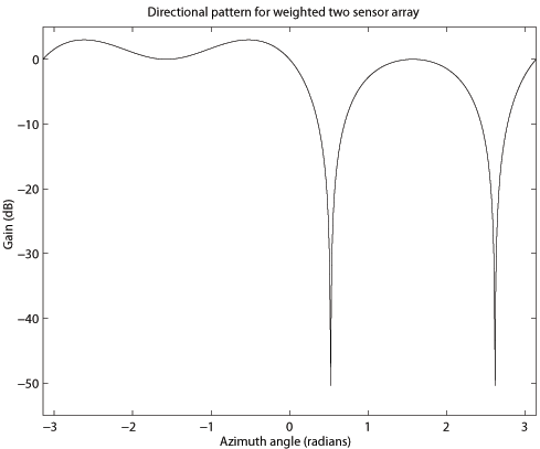
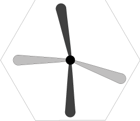
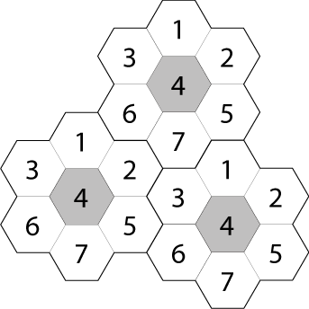
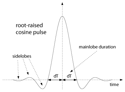
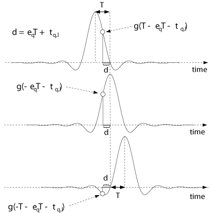
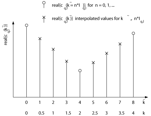
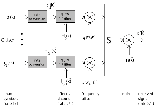
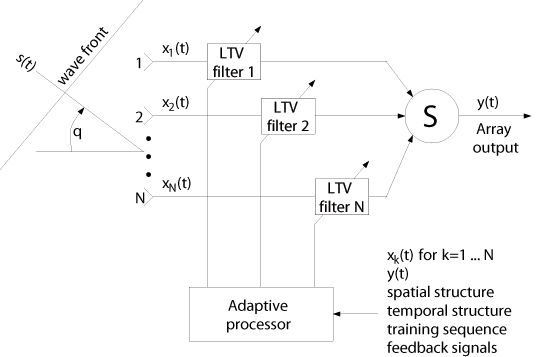
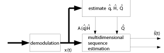
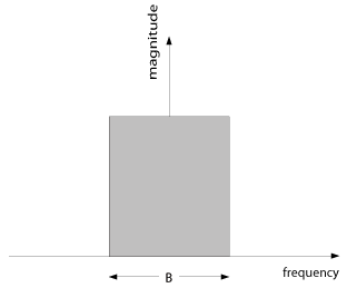
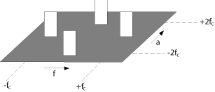
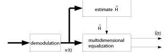