We start out the capacity analysis by reviewing the well known results for the C-CSI channel. In [14]
it is shown that the channel capacity slope increase can be proportional to the number of antennas located at both the input and output of the channel.

Figure 3: Capacity of 1 ×1 and 4 ×4 QAM Systems.
This is illustrated in Figure 3 for 1 ×1 and 4 ×4 flat fading MIMO systems and several different QAM alphabets with the capacity shown,
in the usual way, as a function of the SNR. In the following we would like to examine how the principle of DA channel estimation affects the capacity of such
flat fading MIMO systems. We recall that in the previous Sections of this paper it was shown that channel capacity is a function of the channel dynamics through
LMMSE channel estimation which itself turned out to be a by-product of the capacity derivation. Specifically, it was shown that the total achievable rate over a
flat fading MIMO channel is given by
which can be calculated by evaluating eq. (9) via Monte Carlo simulation. The mutual information I(z;A|zP,AP) is a function of F, the Doppler frequency of the channel fading processes, 1/L, the channel sampling rate, and the SNR. Due to pilot symbol insertion the total amount of usable data symbols is N-NP. Since each channel coefficient is sampled with a rate 1/L, the fraction of the channel capacity available to data transmission is given by
The assumption that the channel must be sampled at least with Nyquist rate, in order to guarantee that the channel trajectory can be reconstructed properly, results in the constraint
The results presented so far enable us to compute channel capacity with respect to the channel sampling rate. Figures 4 to 5 show the result of the Monte Carlo simulations for 1 ×1, and 4 ×4 systems, plotting channel capacity versus channel sampling period L for several typical SNR's and Doppler frequencies (SNR = {0, 6, 12 dB}, F = {0.005, 0.01, 0.02, 0.05 }). The simulations presented here assume an M-ary communication system with QAM modulation (M=16 was used to produce Figures 4 and 5), and equally probable symbol vectors, i.e. p(Ak) = 1/MT. Capacity curves are only shown for channel sampling periods L up to the Nyquist rate.

Figure 4: Capacity of 1 ×1 System.
For the 1 ×1 system depicted in Figure 4, inspection of the results reveals that all capacity curves exhibit a distinct maximum for channel sampling periods strictly smaller than Nyquist sampling (i.e. L < 0.5/F). Two opposing effects are at work here: For very small L, the channel estimates have a very small MSE, so that I(z;A|zP,AP) is close to the mutual information of a perfectly known (C-CSI) channel. In order to achieve such a small MSE, however, a large portion of the channel capacity is sacrificed to the insertion of pilot symbols (the scaling factor [(L-T)/L] of equation (32)). For very large L approaching Nyquist sampling, the capacity is reduced not primarily due to inserted pilot symbols, but the increased MSE of the channel estimates directly reduces the mutual information I(z;A|zP,AP) as shown in Section 3 of the paper. This also explains why a higher SNR shifts the maximum of the capacities to higher L. Further inspection of the simulation results indicate clearly that for smaller Doppler frequencies the capacity difference between the optimal L and Nyquist rate sampling is much larger than for the larger Doppler frequencies. In that sense, an optimal choice of L is much more important for a slow fading channel than for a fast fading channel, because potential capacity losses are larger. For perfectly known (C-CSI) channels, the capacity of the MIMO systems scales linearly with the number of antenna pairs, as demonstrated in Figure 3. In order to see whether the same holds true for MIMO systems with DA channel estimation, Figure 5 shows the results for the 4 ×4 systems, and the 1 ×1 system scaled by 4. The Figure demonstrates that for small Doppler frequencies capacity scales almost linearly, whereas for increasingly larger Doppler frequencies capacity eventually degrades substantially. It is noted that in general the optimal capacities are achieved for the 4 ×4 system at significantly higher channel sampling periods L than for the 1 ×1 system. This is plausible, since for larger numbers of transmit antennas T, more pilot symbol vectors are required in order to sample the channel adequately. Consequently, the factor [(L-T)/L] of equation (32) results in a much reduced capacity, especially at lower channel sampling periods L, as compared to the 1 ×1 case. At higher Doppler frequencies and higher SNRs this leads to the fact that capacity continuously increases up to the Nyquist sampled channel. This observation led us to examine more closely what happens to channel capacity when the channel is actually undersampled. Here we focused on the largest Doppler frequency F=0.05, and the result is presented in Figure 6. For channel sampling periods L = 0, 1, ¼, [0.5/F]=10, the curve is identical to the corresponding curve in Figure 5.

Figure 5: Capacity of 4 ×4 System.
Thereafter, L increases in steps of T=4 such that L = 12, 16, ¼, 48. A step-size equal to the number of transmit antennas T=4 was chosen in order to use a regular distribution for the pilot symbols. An irregular distribution would complicate things further, because for an undersampled channel, the MSE of the channel estimates depends on the relative time index i at which we wish to interpolate the channel (see also Section 4). This implies that the pattern used to insert the pilots matters and should be optimized, since mutual information I(z;A|zP,AP) is higher at relative time indices which correspond to a smaller MSE. From the capacity curves of Figure 6 we draw the conclusion that undersampling the channel, at least in the setup considered here, does not result in a larger capacity than sampling the channel with Nyquist rate. This is due to the fact that once aliasing occurs, the MSE of the channel estimates increases sharply, and thus further reduces the capacity, even though fewer pilot symbols are used.
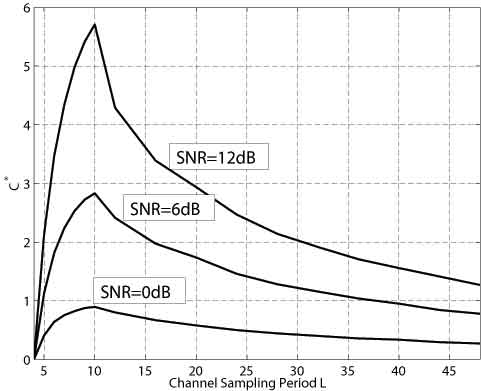
Figure 6: Capacity of 4 ×4 System.
The effect of aliasing on the MSE is illustrated in Figure 7, for a Doppler frequency of F=0.05, and a channel variance sh2 = 1. For purposes of illustration, the Figure shows the MSE averaged over the relative time index i, i.e. se2 = [1/(F-1)] åi=1F-1 se;nL+i2 (see also Section 4). Of course, when computing the mutual information I(z;A|zP,AP), we cannot use the averaged MSE of Figure 7, but have to compute mutual information for each relative time index i = 1, ¼, F-1, and average the result.

Figure 7: Mean square error se2 of Channel Estimate vs L.
