Abstract
The capacity of a coded modulation (CM) digital communication system following the principle of synchronized detection is derived under the assumption that the system operates on a flat fading multiple input-multiple output (MIMO) channel and uses an interleaver to combat bursty error events. It is shown that linear minimum mean square error (LMMSE) channel estimation is an outcome of the capacity derivation, and links channel capacity to the channel dynamics. Based on the assumption that known pilot symbols are transmitted, the channel capacity is optimized with respect to the amount of pilot information needed.
1 INTRODUCTION
Due to complexity constraints, virtually all of todays digital wireless communication systems follow the principle of synchronized detection for which a channel estimate [^h] is formed and subsequently used for detection as if it were the true known channel. Furthermore, we assume that known pilot symbols are transmitted in order to estimate the channel. Usually, the performance of such a communication system is estimated by assuming that the channel estimation error translates directly into a simple signal-to-noise-ratio (SNR) loss. While this approach has proven very useful when designing communication systems, the interesting question of how the principle of synchronized detection affects the achievable capacity is still largely unanswered, although similar problems have been treated in the literature and [13] gives a good overview of the area. In [10], for example, the capacity of a system with a fixed, modified nearest-neighbor decoding rule is analyzed with respect to errors in the estimation of the channel fading process. Here, since we make no assumption on the decoding rule, optimal decoding is implied. Similar problems are also treated in [11] and [12]. However, even if these papers consider a similar problem, the approach taken is entirely different. Here, the mutual information of a flat fading communication system with perfect interleaving is computed, whereas [11] derives capacity bounds for a channel without interleaver, and [12] uses these bounds in the framework of MIMO block-fading channels. Furthermore, it is shown here that the MMSE channel estimator and the corresponding mean square error are results of the capacity derivation, whereas in [11] channel estimation is introduced in an ad-hoc fashion and not an outcome of the derivation. The quantitative results presented here assume a time-varying (Rayleigh fading) channel model unlike the block-fading model used in [12]. In this paper, which is essentially the extension of [7] from the single input-single output (SISO) the multiple input-multiple output (MIMO) case, the capacity is computed for a typical coded modulation (CM) transmission system operating on flat fading MIMO channels and using an interleaver to combat bursty error events. It is shown that the channel capacity is a function of the channel dynamics through linear minimum mean square error (LMMSE) channel estimation which turns out to be a by-product of the capacity derivation. This result can be used to optimize capacity with respect to the amount of pilot information needed for a given scenario in terms of channel dynamics and the SNR.
2 CHANNEL MODEL
| | Figure 1: MIMO Transmission System with Synchronized Detection. |
A CM transmission system operating on a flat-fading MIMO channel and featuring data-aided (DA) synchronized detection is shown in Figure 1. In the transmitter, the signal is encoded, interleaved, and pilot symbols are inserted. For synchronized detection the inner receiver performs DA channel estimation and delivers the estimated channel coefficients and the received symbols to the outer receiver. The outer transmission system thus comprises channel coding, modulation (symbol mapping), interleaving/deinterleaving, and decoding. The interleaving/deinterleaving is employed to transform the bursty channel into a channel having independent errors. This is necessary, since most well-known codes have been devised to combat statistically independent errors.
We assume a flat fading channel which is characterized by the number of transmit antennas T and the number of receive antennas R. In the following such systems are referred to as R ×T MIMO systems. For the encoded and interleaved data symbols ak¢ a linear transmission model results where at time instance k a received signal vector zk¢ depends on a R ×T channel matrix Hk¢. Equivalently, one can also use a R ×RT transmit signal matrix Ak¢ and a RT ×1 channel vector hk¢. Even though this second representation is less intuitive, it is better suited for the subsequent derivations, and we will therefore use it throughout the paper.
The additive complex Gaussian noise at the different receive antenna elements is assumed to be independent, i.e. we have E{mk¢mk¢H} = N0 ·I. Furthermore, the entries hl;k¢ of the channel vector hk¢ are modeled as stationary, zero mean, circularly symmetric complex Gaussian processes of variance sh2 and Doppler spectrum S(ej w). This choice models a Rayleigh fading environment with enough separation of the receiving antenna elements such that the fades for each transmit-receive antenna pair are independent. Furthermore, unity symbol power is assumed throughout, i.e. E{ak¢Hak¢} = 1, and hence the average SNR is given by [`(g)]s = sh2/N0.
For purposes of DA channel estimation, it is assumed that, on average, NP known pilot symbol vectors { aP;k } per ND data symbol vectors are multiplexed into the interleaved data stream. For the received pilot symbol vectors, the following transmission model results
Based on the received pilot symbols, the DA channel estimation produces estimates {[^(h)]k¢} of the fading process {hk¢}. Both, the channel estimates and the received data symbols are passed to the de-interleaver which maps {zk¢} ® {zk} and {[^(h)]k¢} ® {[^(h)]k}. If we assume an ideal interleaving/de-interleaving operation which produces independent received data symbols then the mapping {zk¢} ® {zk} results in the following channel model
where now the individual fading processes hl;k of the channel vector hk are spectrally white. The entire sequence of NP received pilot symbol vectors, denoted with the R ·NP ×1 vector zP, is the given by
Similarly, the received data symbol vectors are stacked in z, and the corresponding transmitted data, channel, and noise are written as A, h, and m, respectively.
3 CAPACITY DERIVATION
In this Section, the capacity for the aforementioned channel model is derived. Since the transmission model assumes the usage of pilot symbols in order to estimate the channel, the channel is said to be partially known to the receiver. We denote this channel P-CSI. In contrast, if complete (perfect) channel knowledge is available, we choose to use C-CSI. The P-CSI channel described in the previous Section, with inputs {A, AP} and outputs {z, zP}, is completely characterized by the distribution p(z,zP | A,AP). Hence, for a given symbol constellation, and under the constraint of identically distributed symbols, the capacity of this channel is given by the mutual information I(z,zP;A,AP). Mutual information is measured in bits per channel use, where one channel use refers here to a block of N=ND+NP transmitted symbol vectors, of which ND are usable data symbols vectors. Therefore, the achievable rate over such a channel per transmitted symbol vector is given by
Compare this to the capacity of the C-CSI channel which is given by [9].
Now, according to the chain rule for mutual information we can rewrite I(z,zP;A,AP) as follows
| | | | | | I(zP;A,AP) + I(z;A,AP | zP) |
| (7) |
|
Since zP does not convey any information about A, the first term reduces to I(zP;AP). If, furthermore, AP is a completely known (nonrandom) pilot matrix, then only the second term of equation (7) remains, and, applying the chain rule again, we get
| | | | | | | I(z;A | AP , zP) +I(z;AP | zP) |
| | | | (8) |
|
Having that in mind, it is possible to write
| | | I(z,zP;A,AP) = I(z;A | AP , zP) = |
| | | | Ez,zP,A | ì
í
î | log | p(z |A,AP,zP)
| | ü
ý
þ | |
| (9) |
|
Note, that since AP is the known pilot matrix, the expectation does not have to be taken with respect to AP. The channel characterized by the distribution p(z | A,AP,zP) is not memoryless, because the fading co-efficients are not perfectly known to the receiver. Therefore, in general, the received data symbol vectors { zk } are not independent. However, with an ideal interleaving/de-interleaving operation that completely breaks up the channel memory, and for a finite-index set N we can write [6] (The effect of the interleaver/de-interleaver on mutual information is outlined in more detail in the Appendix).
| p(z | A,AP,zP) = |
Õ
k Î N | p(zk | Ak, AP,zP) |
| (10) |
In other words, for a block of N=ND+NP transmitted symbol vectors, the mutual information for this channel reduces to
| I(z;A | AP , zP) = | ND-1
å
k=0 | I( zk ; Ak | AP , zP ) |
| (11) |
Remembering that our transmission model is given by zk = Akhk + mk, it becomes obvious that zk and zP, conditioned on Ak and AP, are jointly Gaussian. Therefore, p(zk | Ak, AP,zP) is also normally distributed and completely described by its conditional mean and covariance matrix. From estimation theory we know that the conditional mean E{ zk | Ak, AP,zP } is the estimator [^(z)]h of zk in the minimum mean square error (MMSE) sense. Since the channel model is linear and all associated quantities are Gaussian, the corresponding estimator is itself linear. The conditional mean [^(z)]k computes as
where it is recognized that p( hk | AP,zP ) is also Gaussian distributed and therefore E{ hk | AP,zP } is the optimal linear minimum mean square error (LMMSE) channel estimator [^(h)]k. The covariance matrix of p(zk | Ak, AP,zP) is given by
| | | | E{ | ê
ê | zk - | ^
z
|
k | ê
ê | 2
| | Ak, AP,zP } |
| | | | Ak E{ | ê
ê | hk- | ^
h
|
k | ê
ê | 2
| }AkH + I ·N0 |
| | | | (13) |
|
Therefore, the distribution p(zk | Ak, AP,zP) is normal according to
| | | p(zk | Ak, AP,zP) = p(zk | Ak, | ^
h
|
k | ) = |
| | | | | 1
det
| ( Ak Ce;k AkH +I ·N0)pR |
| · |
| | | | exp | ì
í
î | -(zk-Ak | ^
h
|
k | )H(Ak Ce;kAkH +I ·N0)-1 (zk-Ak | ^
h
|
k | ) | ü
ý
þ | |
| | (14) |
|
It is noticed, that this distribution is a function of the error covariance matrix Ce;k = E{|hk-[^(h)]k |2} of the channel estimate which depends on the time index k for which we wish to estimate (interpolate) the channel. It is therefore concluded that the capacity of an interleaved channel is a function of the channel dynamics via LMMSE channel estimation and the corresponding error covariance matrix. Channel estimation and its relationship to channel dynamics is elaborated in detail in the next Section of this paper.
With these results in mind, it is now possible to formulate an equivalent transmission model, based on the channel estimate [^(h)]k and a noise process [`(m)]k which is distributed according to p(zk | Ak, [^(h)]k), i.e. we have
| | | | | | | Ak | ^
h
|
k | + Ak | æ
è | hk- | ^
h
|
k | ö
ø | + mk |
| | | | | | | (15) |
|
Since [^(h)]k is a linear combination of the Gaussian variables of zP, it is too Gaussian [4]. The corresponding mean and covariance matrix are given by
The first result is due to the zero mean channel and the fact that for the LMMSE estimator the mean of the error is zero [4], and the latter result is a consequence of the orthogonality principle. In summary, two effects influence the capacity:
- the AWGN process {[`(m)]k} has a higher variance than the channel AWGN {mk}, which leads to an effective loss in SNR
- the optimal LMMSE estimator [^(h)]k delivers channel estimates that are orthogonal to the estimation error. This implies, that the estimated channel has a lower variance than the true channel which, again, leads to an additional effective SNR loss.
4 CHANNEL ESTIMATION
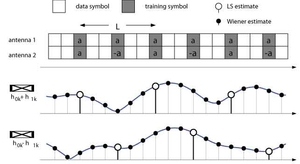
| | Figure 2: MIMO Channel Estimation Example. |
In the previous Section it was shown, that LMMSE channel estimation is a by-product when deriving the capacity C*P-CSI of the synchronized detection channel. In a receiver, LMMSE channel estimation would be performed in the so-called inner receiver, as illustrated by Figure 1. For the purpose of channel estimation, known pilot symbol vectors aP;k are inserted into the interleaved data message. In an R ×T MIMO system, a total of R ·T channel coefficients have to be estimated. The corresponding LMMSE channel estimator is given by [4,1]
| | | | | | | Rhk¢hPHAPH(APRhPAPH+RmP)-1zP |
| (17) |
|
with Rhk¢hP = E{hk¢hPH}, RhP = E{hPhPH}, and RmP = E{mPmPH}. Invoking the matrix inversion lemma twice [1], the estimator can be rewritten as
| | | | ^
h
| ¢
k | = |
Rhk¢hPH(RhP +(APHR-1mPAP)-1)-1
Wk | · |
| | | |
(APHR-1mPAP)-1APHR-1mPzP
hLS;k | |
| (18) |
|
resulting in a Wiener filter Wk applied to the least squares (LS) channel estimate hLS;k. One could also say that the channel is ``sampled'' via a LS estimator and subsequently low-pass filtered with a Wiener filter in order to interpolate the missing channel samples. Note, that the LS channel estimate only exists, if APHR-1mPAP is full rank and thus invertible. If the number of transmit antennas is larger than one, i.e. T > 1, the LS channel estimate does not exist. This is intuitively clear since RT channel coefficients cannot be estimated from R observations without side information. However, it is possible to rewrite the channel model as
with AX = I, and hXP = APhP. Now AX is full rank and the LS estimate of hXP does exist. If, furthermore, the pilot symbol vectors {aP;k} are chosen to be orthogonal with respect to time within one channel sampling period L (see Figure 2), the coefficients of the effective channel hX = Ah are again i.i.d. It is thus possible to apply a Wiener filter to the LS estimate [^(h)]XP in order to perform LMMSE channel estimation of the effective channel hX, i.e. we have
This can also be rewritten in terms of individual Wiener filters
| | ^
h
|
X,l;k | = wX,l;kH | ^
h
|
XP,l | for l = 0, ¼, RT-1 |
| (21) |
where [^(h)]XP,l only contains least squares (LS) channel samples of the l-th effective channel coefficient. The channel estimation process is illustrated by way of example in Figure 2 for a simple system with T=2 transmit antennas and R=1 receive antennas. As shown in the Figure, both resulting effective channel coefficients are sampled with a sampling period of L. Clearly, since orthogonal pilot vectors are used, channel estimates of the true channel can subsequently be computed from the result of the Wiener interpolation via a simple matrix multiplication, i.e.
In our simple example shown in Figure 2, X would be
The quality of the LMMSE channel estimate is characterized by the error covariance Ce;k. If orthogonal pilot vectors, as described above, are used, the error covariance is given by Ce;k = se;k2·I, and we can write
| se;k2 = E{|hl;k¢- | ^
h
| ¢
l;k | |2 } for l = 0, ¼, RT-1 |
| (24) |
The MSE se;k2 is directly related to the channel dynamics via the Doppler spectrum S(ejw) and the channel sampling rate 1/L. As mentioned before, the individual fading processes of the channel vector hk¢ have a Doppler spectrum S(ejw). On mobile channels the U-shaped Jakes Doppler spectrum is often assumed [5]. The Jakes spectrum, which is based on the isotropic scattering assumption, accentuates instantaneous Doppler shifts near the cutoff frequency F (F is normalized to the symbol rate T). However, since the actual shape of the Doppler spectrum has no noticeable effect on the estimator performance [1, pp. 651, 658], for the purpose of the capacity calculations, the Jakes Doppler spectrum may as well be replaced by an ideal lowpass spectrum with the same cutoff frequency F, i.e. we have
Assuming, in an information theoretic framework, an infinite length, equally spaced pilot symbol vector aP, frequency domain Wiener filter theory becomes applicable. Denoting the LS channel estimates {xk}, the Wiener filter {wi;k}, and the channel estimates {[^h]l;k¢}, the channel estimate can be expressed as
| | ^
h
| ¢
l;k | = | ^
h
| ¢
l;nL+i | = | ¥
å
n=-¥ | wi;n xnL-nL |
| (26) |
where k=nL+i is used to indicate that the channel is interpolated at time index i relative to the LS channel samples which are available at time indices nL. Applying the orthogonality principle and the discrete-time Fourier transform, the optimal Wiener filter is given in the frequency domain by
| Wi(ejw) = ej([(w-2pk)/L] )i · | 1
L | | L-1
å
k=0 | S(e[(j(w- 2pk )i)/L]) |
1
L | | L-1
å
k=0 | S(e[(j(w- 2pk )i)/L])+ N0 |
| |
| (27) |
Defining the channel autocorrelation function as a*kL+i=E{ hl;mL-kL¢ hl;mL+i*¢ }, we can compute the MSE se;nL+i2 using the orthogonality principle and applying Parseval's theorem.
| | | se;nL+i2 = E | ì
í
î | | ê
ê | h¢l;nL+i - | ^
h
| ¢
l;nL+i | ê
ê | 2
| ü
ý
þ | = |
| | | | a*0 - | ¥
å
k=-¥ | wi;k a*kL+i = |
| | | | sh2 - | 1
2p | | ó
õ | p
-p | Wi(ejw) | 1
L | | L-1
å
k=0 | e-j([(w-2pk)/L] )iS(e[(j(w- 2pk )i)/L])dw |
| | | | (28) |
|
If the rectangular Doppler spectrum S(ej w) of equation (25) is assumed, and the channel is sampled at least with Nyquist frequency, then the MSE evaluates as [7]
| se;nL+i2 = | 2 F L N0 sh2
2 F L N0 + sh2 | |
| (29) |
In that case the MSE does not depend on the relative time index i (or the absolute time index k) at which we wish to interpolate the channel. This independence is a direct result of applying Parseval's theorem which is invariant to a time shift. Therefore, when computing the capacity C*P-CSI, no additional averaging over the different mean square errors is necessary. However, if the channel is undersampled, the MSE of the channel estimates, in general, depends on the relative time index i, and it can be obtained by numerically evaluating eq. (28).
Finally, note that equations (28) and (29) refer to the MSE of the channel estimates for the channel vector h¢k which is characterized by its Doppler Spectrum S(ej w). Since the de-interleaver maps {[^(h)]k¢} ® {[^(h)]k} we have that
| Ce;k = E{|hk- | ^
h
|
k | |2 } = E{|h¢k- | ^
h
| ¢
k | |2 } |
| (30) |
Before the de-interleaver, the entries {[^h]¢l;k} of the channel estimates {[^(h)]¢k} are a colored sequence with power spectrum S(ej w), and after de-interleaving, the white sequence {[^h]l;k} results. Since the pilot symbol vectors are inserted in the transmitter after the interleaver, the received pilots zP;k and the received data zk¢ are correlated via S(ej w), whereas the de-interleaver has destroyed any correlation between the received data symbol vectors zk.